C is a simple language. You’re only allowed to have one function with each name. C++, on the other hand, gives you much more flexibility:

• You can have multiple functions with the same name (overloading).
• You can overload built-in operators like + and ==.
• You can write function templates.
• Namespaces help you avoid naming conflicts.

I like these C++ features. With these features, you can make str1 + str2 return the concatenation of two strings. You can have a pair of 2D points, and another pair of 3D points, and overload dot(a, b) to work with either type. You can have a bunch of array-like classes and write a single sort function template that works with all of them.

But when you take advantage of these features, it’s easy to push things too far. At some point, the compiler might unexpectedly reject your code with errors like:

error C2666: 'String::operator ==': 2 overloads have similar conversions
note: could be 'bool String::operator ==(const String &) const'
note: or       'built-in C++ operator==(const char *, const char *)'
note: while trying to match the argument list '(const String, const char *)'

Like many C++ programmers, I’ve struggled with such errors throughout my career. Each time it happened, I would usually scratch my head, search online for a better understanding, then change the code until it compiled. But more recently, while developing a new runtime library for Plywood, I was thwarted by such errors over and over again. It became clear that despite all my previous experience with C++, something was missing from my understanding and I didn’t know what it was.

Fortunately, it’s now 2021 and information about C++ is more comprehensive than ever. Thanks especially to cppreference.com, I now know what was missing from my understanding: a clear picture of the hidden algorithm that runs for every function call at compile time.

This is how the compiler, given a function call expression, figures out exactly which function to call:

may performargument-dependentlookup may involveSFINAE non-templatefunction functiontemplate finds implicitconversions candidatefunctions viablefunctions TIEBREAKERS Template argumentdeduction Template argumentsubstitution Arguments mustbe compatible Constraints mustbe satisfied (C++20) Better-matching arguments wins Non-template function wins More specialized template wins additional tiebreakers otherwise Overload Resolution NameLookup Special Handling ofFunction Templates Unqualifiedname lookup Qualifiedname lookup Membername lookup

These steps are enshrined in the C++ standard. Every C++ compiler must follow them, and the whole thing happens at compile time for every function call expression evaluated by the program. In hindsight, it’s obvious there has to be an algorithm like this. It’s the only way C++ can support all the above-mentioned features at the same time. This is what you get when you combine those features together.

I imagine the overall intent of the algorithm is to “do what the programmer expects”, and to some extent, it’s successful at that. You can get pretty far ignoring the algorithm altogether. But when you start to use multiple C++ features, as you might when developing a library, it’s better to know the rules.

So let’s walk through the algorithm from beginning to end. A lot of what we’ll cover will be familiar to experienced C++ programmers. Nonetheless, I think it can be quite eye-opening to see how all the steps fit together. (At least it was for me.) We’ll touch on several advanced C++ subtopics along the way, like argument-dependent lookup and SFINAE, but we won’t dive too deeply into any particular subtopic. That way, even if you know nothing else about a subtopic, you’ll at least know how it fits into C++’s overall strategy for resolving function calls at compile time. I’d argue that’s the most important thing.

Name Lookup

Our journey begins with a function call expression. Take, for example, the expression blast(ast, 100) in the code listing below. This expression is clearly meant to call a function named blast. But which one?

namespace galaxy {
    struct Asteroid {
        float radius = 12;
    };
    void blast(Asteroid* ast, float force);
}

struct Target {
    galaxy::Asteroid* ast;
    Target(galaxy::Asteroid* ast) : ast{ast} {}
    operator galaxy::Asteroid*() const { return ast; }
};

bool blast(Target target);
template <typename T> void blast(T* obj, float force);

void play(galaxy::Asteroid* ast) {
    blast(ast, 100);
}

The first step toward answering this question is name lookup. In this step, the compiler looks at all functions and function templates that have been declared up to this point and identifies the ones that could be referred to by the given name.

As the flowchart suggests, there are three main types of name lookup, each with its own set of rules.

• Member name lookup occurs when a name is to the right of a . or -> token, as in foo->bar. This type of lookup is used to locate class members.
• Qualified name lookup occurs when a name has a :: token in it, like std::sort. This type of name is explicit. The part to the right of the :: token is only looked up in the scope identified by the left part.
• Unqualified name lookup is neither of those. When the compiler sees an unqualified name, like blast, it looks for matching declarations in various scopes depending on the context. There’s a detailed set of rules that determine exactly where the compiler should look.

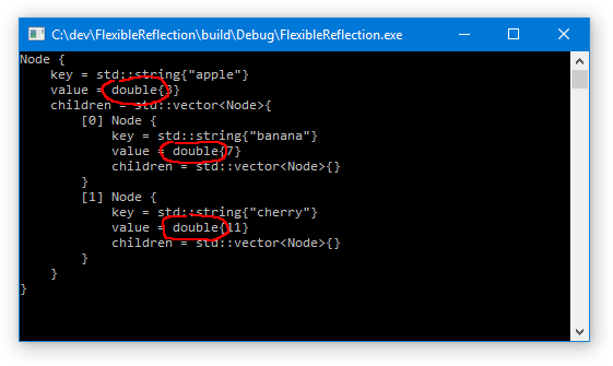
In our case, we have an unqualified name. Now, when name lookup is performed for a function call expression, the compiler may find multiple declarations. Let’s call these declarations candidates. In the example above, the compiler finds three candidates:

The first candidate, circled above, deserves extra attention because it demonstrates a feature of C++ that’s easy to overlook: argument-dependent lookup, or ADL for short. I’ll admit, I spent most of my C++ career unaware of ADL’s role in name lookup. Here’s a quick summary in case you’re in the same boat. Normally, you wouldn’t expect this function to be a candidate for this particular call, since it was declared inside the galaxy namespace and the call comes from outside the galaxy namespace. There’s no using namespace galaxy directive in the code to make this function visible, either. So why is this function a candidate?

The reason is because any time you use an unqualified name in a function call – and the name doesn’t refer to a class member, among other things – ADL kicks in, and name lookup becomes more greedy. Specifically, in addition to the usual places, the compiler looks for candidate functions in the namespaces of the argument types – hence the name “argument-dependent lookup”.

The complete set of rules governing ADL is more nuanced than what I’ve described here, but the key thing is that ADL only works with unqualified names. For qualified names, which are looked up in a single scope, there’s no point. ADL also works when overloading built-in operators like + and ==, which lets you take advantage of it when writing, say, a math library.

Interestingly, there are cases where member name lookup can find candidates that unqualified name lookup can’t. See this post by Eli Bendersky for details about that.

Special Handling of Function Templates

Some of the candidates found by name lookup are functions; others are function templates. There’s just one problem with function templates: You can’t call them. You can only call functions. Therefore, after name lookup, the compiler goes through the list of candidates and tries to turn each function template into a function.

In the example we’ve been following, one of the candidates is indeed a function template:

This function template has a single template parameter, T. As such, it expects a single template argument. The caller, blast(ast, 100), didn’t specify any template arguments, so in order to turn this function template into a function, the compiler has to figure out the type of T. That’s where template argument deduction comes in. In this step, the compiler compares the types of the function arguments passed by the caller (on the left in the diagram below) to the types of the function parameters expected by the function template (on the right). If any unspecified template arguments are referenced on the right, like T, the compiler tries to deduce them using information on the left.

In this case, the compiler deduces T as galaxy::Asteroid because doing so makes the first function parameter T* compatible with the argument ast. The rules governing template argument deduction are a big subject in and of themselves, but in simple examples like this one, they usually do what you’d expect. If template argument deduction doesn’t work – in other words, if the compiler is unable to deduce template arguments in a way that makes the function parameters compatible with the caller’s arguments – then the function template is removed from the list of candidates.

Any function templates in the list of candidates that survive up to this point are subject to the next step: template argument substitution. In this step, the compiler takes the function template declaration and replaces every occurrence of each template parameter with its corresponding template argument. In our example, the template parameter T is replaced with its deduced template argument galaxy::Asteroid. When this step succeeds, we finally have the signature of a real function that can be called – not just a function template!

Of course, there are cases when template argument substitution can fail. Suppose for a moment that the same function template accepted a third argument, as follows:

template <typename T> void blast(T* obj, float force, typename T::Units mass = 5000);

If this was the case, the compiler would try to replace the T in T::Units with galaxy::Asteroid. The resulting type specifier, galaxy::Asteroid::Units, would be ill-formed because the struct galaxy::Asteroid doesn’t actually have a member named Units. Therefore, template argument substitution would fail.

When template argument substitution fails, the function template is simply removed from the list of candidates – and at some point in C++’s history, people realized that this was a feature they could exploit! The discovery led to a entire set of metaprogramming techniques in its own right, collectively referred to as SFINAE (substitution failure is not an error). SFINAE is a complicated, unwieldy subject that I’ll just say two things about here. First, it’s essentially a way to rig the function call resolution process into choosing the candidate you want. Second, it will probably fall out of favor over time as programmers increasingly turn to modern C++ metaprogramming techniques that achieve the same thing, like constraints and constexpr if.

Overload Resolution

At this stage, all of the function templates found during name lookup are gone, and we’re left with a nice, tidy set of candidate functions. This is also referred to as the overload set. Here’s the updated list of candidate functions for our example:

The next two steps narrow down this list even further by determining which of the candidate functions are viable – in other words, which ones could handle the function call.

Perhaps the most obvious requirement is that the arguments must be compatible; that is to say, a viable function should be able to accept the caller’s arguments. If the caller’s argument types don’t match the function’s parameter types exactly, it should at least be possible to implicitly convert each argument to its corresponding parameter type. Let’s look at each of our example’s candidate functions to see if its parameters are compatible:

Candidate 1

The caller’s first argument type galaxy::Asteroid* is an exact match. The caller’s second argument type int is implicitly convertible to the second function parameter type float, since int to float is a standard conversion. Therefore, candidate 1’s parameters are compatible.

Candidate 2

The caller’s first argument type galaxy::Asteroid* is implicitly convertible to the first function parameter type Target because Target has a converting constructor that accepts arguments of type galaxy::Asteroid*. (Incidentally, these types are also convertible in the other direction, since Target has a user-defined conversion function back to galaxy::Asteroid*.) However, the caller passed two arguments, and candidate 2 only accepts one. Therefore, candidate 2 is not viable.

void galaxy::blast(galaxy::Asteroid* ast, float force) bool blast(Target target) void blast<galaxy::Asteroid>(galaxy::Asteroid* obj, float force) 2 1 3

Candidate 3

Candidate 3’s parameter types are identical to candidate 1’s, so it’s compatible too.

Like everything else in this process, the rules that control implicit conversion are an entire subject on their own. The most noteworthy rule is that you can avoid letting constructors and conversion operators participate in implicit conversion by marking them explicit.

After using the caller’s arguments to filter out incompatible candidates, the compiler proceeds to check whether each function’s constraints are satisfied, if there are any. Constraints are a new feature in C++20. They let you use custom logic to eliminate candidate functions (coming from a class template or function template) without having to resort to SFINAE. They’re also supposed to give you better error messages. Our example doesn’t use constraints, so we can skip this step. (Technically, the standard says that constraints are also checked earlier, during template argument deduction, but I skipped over that detail. Checking in both places helps ensure the best possible error message is shown.)

Tiebreakers

At this point in our example, we’re down to two viable functions. Either of them could handle the original function call just fine:

Indeed, if either of the above functions was the only viable one, it would be the one that handles the function call. But because there are two, the compiler must now do what it always does when there are multiple viable functions: It must determine which one is the best viable function. To be the best viable function, one of them must “win” against every other viable function as decided by a sequence of tiebreaker rules.

TIEBREAKERS Better-matching parameters wins Non-template function wins More specialized template wins additional tiebreakers otherwise otherwise otherwise viablefunctions

Let’s look at the first three tiebreaker rules.

First tiebreaker: Better-matching parameters wins

C++ places the most importance on how well the caller’s argument types match the function’s parameter types. Loosely speaking, it prefers functions that require fewer implicit conversions from the given arguments. When both functions require conversions, some conversions are considered “better” than others. This is the rule that decides whether to call the const or non-const version of std::vector’s operator[], for example.

In the example we’ve been following, the two viable functions have identical parameter types, so neither is better than the other. It’s a tie. As such, we move on to the second tiebreaker.

Second tiebreaker: Non-template function wins

If the first tiebreaker doesn’t settle it, then C++ prefers to call non-template functions over template functions. This is the rule that decides the winner in our example; viable function 1 is a non-template function while viable function 2 came from a template. Therefore, our best viable function is the one that came from the galaxy namespace:

void galaxy::blast(galaxy::Asteroid* ast, float force) WINNER!

It’s worth reiterating that the previous two tiebreakers are ordered in the way I’ve described. In other words, if there was a viable function whose parameters matched the given arguments better than all other viable functions, it would win even if it was a template function.

Third tiebreaker: More specialized template wins

In our example, the best viable function was already found, but if it wasn’t, we would move on to the third tiebreaker. In this tiebreaker, C++ prefers to call “more specialized” template functions over “less specialized” ones. For example, consider the following two function templates:

template <typename T> void blast(T obj, float force);
template <typename T> void blast(T* obj, float force);

When template argument deduction is performed for these two function templates, the first function template accepts any type as its first argument, but the second function template accepts only pointer types. Therefore, the second function template is said to be more specialized. If these two function templates were the only results of name lookup for our call to blast(ast, 100), and both resulted in viable functions, the current tiebreaker rule would cause the second one to be picked over the first one. The rules to decide which function template is more specialized than another are yet another big subject.

Even though it’s considered more specialized, it’s important to understand that the second function template isn’t actually a partial specialization of the first function template. On the contrary, they’re two completely separate function templates that happen to share the same name. In other words, they’re overloaded. C++ doesn’t allow partial specialization of function templates.

There are several more tiebreakers in addition to the ones listed here. For example, if both the spaceship <=> operator and an overloaded comparison operator such as > are viable, C++ prefers the comparison operator. And if the candidates are user-defined conversion functions, there are other rules that take higher priority than the ones I’ve shown. Nonetheless, I believe the three tiebreakers I’ve shown are the most important to remember.

Needless to say, if the compiler checks every tiebreaker and doesn’t find a single, unambiguous winner, compilation fails with an error message similar to the one shown near the beginning of this post.

After the Function Call Is Resolved

We’ve reached the end of our journey. The compiler now knows exactly which function should be called by the expression blast(ast, 100). In many cases, though, the compiler has more work to do after resolving a function call:

• If the function being called is a class member, the compiler must check that member’s access specifiers to see if it’s accessible to the caller.
• If the function being called is a template function, the compiler attempts to instantiate that template function, provided its definition is visible.
• If the function being called is a virtual function, the compiler generates special machine instructions so that the correct override will be called at runtime.

None of those things apply to our example. Besides, they’re outside the scope of this post.

This post didn’t contain any new information. It was basically a condensed explanation of an algorithm already described by cppreference.com, which, in turn, is a condensed version of the C++ standard. However, the goal of this post was to convey the main steps without getting dragged down into details. Let’s take a look back to see just how much detail was skipped. It’s actually kind of remarkable:

• There’s an entire set of rules for unqualified name lookup.
• Within that, there’s a set of rules for argument-dependent lookup.
• Member name lookup has its own rules, too.
• There’s a set of rules for template argument deduction.
• There’s an entire family of metaprogramming techniques based on SFINAE.
• There’s a set of rules governing how implicit conversions work.
• Constraints (and concepts) are a completely new feature in C++20.
• There’s a set of rules to determine which implicit conversions are better than others.
• There’s a set of rules to determine which function template is more specialized than another.

Yeah, C++ is complicated. If you’d like to spend more time exploring these details, Stephan T. Lavavej produced a very watchable series of videos on Channel 9 back in 2012. Check out the first three in particular. (Thanks to Stephan for reviewing an early draft of this post.)

Now that I’ve learned exactly how C++ resolves a function call, I feel more competent as a library developer. Compilation errors are more obvious. I can better justify API design decisions. I even managed to distill a small set of tips and tricks out of the rules. But that’s a subject for another post.

Flap Hero is a small game written entirely in C++ without using an existing game engine. All of its source code is available on GitHub. I think it can serve as an interesting resource for novice and intermediate game developers to study.

In this post, I’ll explain how Flap Hero’s code is organized, how it differs from larger game projects, why it was written that way, and what could have been done better.

Very little information in this post is specific to C++. Most of it would still be relevant if Flap Hero was written in another language like C#, Rust or plain C. That said, if you browse (or build) the source code, you will need some fluency in C++. Learn C++ and Learn OpenGL are two great resources for beginners. For the most part, Flap Hero’s source code sticks to a fairly straightforward subset of C++, but the deeper you go into its low-level modules (like runtime), the more you’ll encounter advanced C++ features like templates and SFINAE.

General Architecture

Flap Hero was developed using Plywood, a C++ framework that helps organize code into reusable modules. Each yellow box in the diagram below represents a Plywood module. The blue arrows represent dependencies.

The biggest chunk of Flap Hero’s game code is located in the flapGame module, which contains roughly 6400 physical lines of code. The two most important source files in the flapGame module are GameFlow.cpp and GameState.cpp.

All the state for a single gameplay session is held inside a single GameState object. This object is, in turn, owned by a GameFlow object. The GameFlow can actually own two GameState objects at a given time, with both gameplay sessions updating concurrently. This is used to achieve an animated “split screen” effect during the transition from one gameplay session to the next.

The flapGame module is meant to be incorporated into a main project. On desktop operating systems, the main project is implemented by the glfwFlap module. The glfwFlap module is responsible for initializing the game’s OpenGL context and for passing input and update events to flapGame. (Android and iOS use completely different main projects, but those serve the same purpose as glfwFlap.) glfwFlap communicates with flapGame using an API defined in a single file: Public.h. There are only 13 functions in this API, and not all of them are used on every platform.

As Few Subsystems As Possible

Flap Hero is not based on an existing game engine. It’s just a C++ program that, when you run it, plays Flap Hero! As such, it doesn’t contain many of the subsystems found in a typical game engine. This was a deliberate choice. Flap Hero is a sample application, and I wanted to implement it using as little code as possible.

What do I mean by “subsystem”? I’ll give a few examples in the following sections. In some cases, it was OK to not have the subsystem; in other cases, it turned out to be a disadvantage. I’ll give a verdict for each one as we go.

No Abstract Scene Representation

In a typical game engine, there’s an intermediate representation of the 3D (or 2D) scene consisting of a bunch of abstract objects. In Godot, those objects inherit from Spatial; in Unreal, they’re AActor instances; in Unity, they’re GameObject instances. All of these objects are abstract, meaning that the details of how they’re rendered to the screen are filled in by subclasses or components.

One benefit of this approach is that it lets the renderer perform view frustum culling in a generic way. First, the renderer determines which objects are visible, then it effectively tells those objects to draw themselves. Ultimately, each object issues a series of draw calls to the underlying graphics API, whether it’s OpenGL, Metal, Direct3D, Vulkan or something else.

Flap Hero has no such scene representation. In Flap Hero, rendering is performed using a dedicated set of functions that issue OpenGL calls directly. Most of the interesting stuff happens in the renderGamePanel() function. This function draws the bird, then the floor, then the pipes, then the shrubs, the cities in the background, the sky, the clouds, particle effects, and finally the UI layer. That’s it. No abstract objects are involved.

For a game like Flap Hero, where the contents of the screen are similar every frame, this approach works perfectly fine.

Verdict: OK

Obviously, this approach has its limitations. If you’re making a game involving exploration, where the contents of the screen can differ greatly from one moment to the next, you’re going to want some kind of abstract scene representation. Depending on the style of game, you could even take a hybrid approach. For example, to make Flap Hero draw different obstacles instead of just pipes, you could replace the code that draws pipes with code that draws a collection of arbitrary objects. The rest of the renderGamePanel() function would remain the same.

No Shader Manager

Since the original Xbox, every game engine I’ve worked on has included some kind of shader manager. A shader manager allows game objects to refer to shader programs indirectly using some sort of “shader key”. The shader key typically describes which features are needed to render each mesh, whether it’s skinning, normal mapping, detail texturing or something else. For maximum flexibility, shader inputs are often passed to the graphics API automatically using some kind of reflection system.

Flap Hero has none of that. It has only a fixed set of shader programs. Shaders.cpp contains the source code for 15 shaders, and Text.cpp contains 2 more. There’s a dedicated shader for the pipes, another for the smoke cloud particles, a couple that are only used in the title screen. All shaders are compiled at startup.

Moreover, in Flap Hero, all shader parameters are managed by hand. What does that mean? It means that the game extracts the locations of all vertex attributes and uniform variables using code that is written by hand for each shader. Similarly, when the shader is used for drawing, the game passes uniform variables and configures vertex attributes using code written by hand for each shader.

    matShader->vertPositionAttrib =
        GL_NO_CHECK(GetAttribLocation(matShader->shader.id, "vertPosition"));
    PLY_ASSERT(matShader->vertPositionAttrib >= 0);
    matShader->vertNormalAttrib =
        GL_NO_CHECK(GetAttribLocation(matShader->shader.id, "vertNormal"));
    PLY_ASSERT(matShader->vertNormalAttrib >= 0);
    ...

This approach became really tedious after the 16th or 17th shader.

Verdict: Bad

I found myself really missing the shader manager I had developed for my custom game engine, which uses runtime reflection to automatically configure vertex attributes and pass uniform variables. In other words, it takes care of a lot of “glue code” automatically. The main reason why I didn’t use a similar system in Flap Hero is because again, Flap Hero is a sample application and I didn’t want to bring in too much extra machinery.

Incidentally, Flap Hero uses the glUniform family of OpenGL functions to pass uniform variables to shaders. This approach is old-fashioned but easy to implement, and helps catch programming errors if you accidentally pass a uniform that the shader doesn’t expect. The more modern approach, which incurs less driver overhead, is to use Uniform Buffer Objects.

No Physics Engine

Many game engines incorporate a physics engine like Bullet, Havok or Box2D. Each of these physics engines uses an approach similar to the “abstract scene representation” described above. They each maintain their own representation of physics objects in a collection known as the physics world. For example, in Bullet, the physics world is represented by a btDiscreteDynamicsWorld object and contains a collection of btCollisionObjects. In Box2D, there’s a b2World containing b2Body objects.

You can almost think of the physics world as a game within a game. It’s more or less self-sufficient and independent of the game engine containing it. As long as the game keeps calling the physics engine’s step function – for example, b2World::Step in Box2D – the physics world will keep running on its own. The game engine takes advantage of the physics world by examining it after each step, using the state of physics objects to drive the position & orientation of its own game objects.

Flap Hero contains some primitive physics, but doesn’t use a physics engine. All Flap Hero needs is to check whether the bird collided with something. For collision purposes, the bird is treated as a sphere and the pipes are treated as cylinders. Most of the work is done by the sphereCylinderCollisionTest() function, which detects sphere-cylinder collisions. The sphere can collide with three parts of the cylinder: the side, the edge or the cap.

For an arcade-style game like Flap Hero that only needs a few basic collision checks, this is good enough. A physics engine isn’t necessary and would have only added complexity to the project. The amount of code needed to integrate a physics engine would likely have been greater than the amount of code needed to perform the collision checks ourselves.

Verdict: Good

Having said that, if you’re working with a game engine that already has an integrated physics engine, it often makes sense to use it. And for games requiring collisions between multiple objects, like the debris in a first-person shooter or the collapsing structures in Angry Birds, physics engines are definitely the way to go.

No Asset Pipeline

By “asset”, I’m referring to data files that are loaded by the game: mainly textures, meshes, animations and sounds. I wrote about asset pipelines in an earlier post about writing your own game engine.

Flap Hero doesn’t have an asset pipeline and has no game-specific formats. Each of its assets is loaded from the format that was used to create it. The game imports 3D models from FBX using Assimp; decodes texture images from PNG using stb_image; loads a TrueType font and creates a texture atlas using stb_truetype; and decodes a 33-second Ogg Vorbis music file using stb_vorbis. All of this happens when the game starts up. Despite the amount of processing, the game still loads fairly quickly.

If Flap Hero had an asset pipeline, most of that processing would be performed ahead of time using an offline tool (often known as the “cooker”) and the game would start even more quickly. But I wasn’t worried about that. Flap Hero is just a sample project, and I didn’t want to introduce additional build steps. In the end, though, I have to admit that the lack of an asset pipeline made certain things more difficult.

Verdict: Bad

If you explore the way materials are associated with 3D meshes in Flap Hero, you’ll see what I mean. For example, the materials used to draw the bird have several properties: diffuse color, specular color, rim light color, specular exponent and rim light falloff. Not all of these properties can be represented in the FBX format. As a result, I ended up ignoring the FBX material properties and defining new materials entirely in code.

With an asset pipeline in place, that wouldn’t be necessary. For example, in my custom game engine, I can define arbitrary material properties in Blender and export them directly to a flexible in-game format. Each time a mesh is exported, the game engine reloads it on-the-fly, even when the game running on a mobile device. This approach is great for iteration times, but obviously takes a lot of work to set up in the first place.

I just released a mobile game called Flap Hero. It’s a Flappy Bird clone with cartoony graphics and a couple of twists: You can go in the pipes (wow!) and it takes two collisions to end the game. Flap Hero is free, quick to download (between 3 - 5 MB) and opens instantly. Give it a try!

Flap Hero is open source, too. Its source code is released under the MIT license and its assets (3D models, sounds, music) are dedicated to the public domain. Do whatever you want with them! Everything’s available on GitHub.

I’m releasing this game to promote Plywood, an open source C++ framework I released a few months ago. Flap Hero was made using Plywood.

How Flap Hero Uses Plywood

If you only read up to this point, you might think that Plywood is a game engine. It isn’t! Plywood is best described as a “module-oriented” C++ framework. It gives you a workspace, a set of built-in modules and some (optional) code generation tricks.

Plywood currently has 36 built-in modules, none of which are specific to game development. For game-specific functionality, Flap Hero relies on several excellent third-party libraries: Assimp to load 3D models, SoLoud for audio, stb to load textures and fonts, and GLFW for desktop windowing & input.

If Flap Hero relies on third-party libraries, you might be wondering, what’s the point of Plywood? Well, those libraries have to be integrated into something. In Plywood, that something is the Plywood workspace. In this workspace, you can create your own modules that depend on other Plywood modules as well as on third-party libraries. You can then instantiate those modules in build folders, and they’ll bring all their dependencies along with them.

In addition to the aforementioned libraries, Flap Hero uses several built-in Plywood modules such as runtime, math and image. Plywood’s runtime module offers an alternative to the standard C and C++ runtimes, providing lean cross-platform I/O, strings, containers and more. The math module provides vectors, matrices, quaternions and other primitives. I’ll continue fleshing out the details of these modules in Plywood’s documentation over time.

A Framework for Efficient Software

Flap Hero is written entirely in C++ and isn’t built on any existing game engine. It keeps bloat to a minimum, resulting in a small download, fast load times, low memory usage, responsive controls and high framerate for the user, even on older devices. This is the “handmade” style of software development championed by communities such as the Handmade Network.

That’s the kind of software that Plywood is meant to help create. Still, Plywood is a work in progress. Here’s what I’d like to do next:

I’m especially excited about the potential of a GUI build manager. The GUI build manager would be a graphical user interface that lets you manage the Plywood workspace interactively, bypassing the somewhat cumbersome command line tool. Ideally, this tool would have close integration with various package managers across different platforms. The goal would be to make it as simple as possible to integrate third-party libraries and get projects built on other machines – something that’s still a bit of a weak spot in Plywood.

The next post on this blog will be a review of Flap Hero’s source code. Stay tuned if that kind of thing interests you!

Plywood is an open-source C++ framework I released a few weeks ago. It includes, among other things, a runtime module that exposes a cross-platform API for I/O, memory, threads, process management and more.

This post is about the I/O part. For those who don’t know, I/O stands for input/output, and refers to the part of a computer system that either writes serialized data to or reads serialized data from an external interface. The external interface could be a storage device, pipe, network connection or any other type of communication channel.

Typically, it’s the operating system’s responsibility to provide low-level I/O services to an application. But there’s still plenty of work that needs to happen at the application level, such as buffering, data conversion, performance tuning and exposing an interface that makes life easier on application programmers. That’s where Plywood’s I/O system comes in.

Of course, standard C++ already comes with its own input/output library, as does the standard C runtime, and most C and C++ programmers are quite familiar with those libraries. Plywood’s I/O system is meant serve as an alternative to those libraries. Those libraries were originally developed in 1984 and the early 1970s, respectively. They’ve stood the test of time incredibly well, but I don’t think it’s outrageous to suggest that, hey, maybe some innovation is possible here.

To be clear, when you build a project using Plywood, you aren’t required to use Plywood’s I/O system – you can still use the standard C or C++ runtime library, if you prefer.

I’m sure this blog post will seem dry for some (or many) readers – but not for me! I like this topic, and I’m willing bet that there are other low-level I/O wonks out there who will find it interesting as well. So let’s jump in.

Writing Raw Bytes to Standard Output

The following program writes "Hello!\n" to standard output as a raw sequence of 7 bytes. No newline conversion or character encoding conversion is performed. Writing takes place through an OutStream, which is a class (defined in the ply namespace) that performs buffered output.

#include <ply-runtime/Base.h>

int main() {
    using namespace ply;
    OutStream outs = StdOut::binary();
    outs.write({"Hello!\n", 7});
    return 0;
}

Now, suppose we pause this program immediately after the OutStream is created, before anything gets written. On a Linux system, this is what the OutStream initially looks like in memory:

1. This is the OutStream object itself. As already mentioned, OutStream is a class that performs buffered output. That means when you write to an OutStream, your data actually gets written to a temporary buffer in memory first.

2. This is the temporary buffer used by the OutStream. OutStream::curByte initially points to the start of this buffer, and OutStream::endByte points to the end. The temporary buffer is 4096 bytes long, as indicated by ChunkListNode::numBytes.

3. This is a ChunkListNode, a reference-counted object that owns the temporary buffer. It’s responsible for freeing the temporary buffer in its destructor. The OutStream holds a reference to this object. (The ability to create additional ChunkListNode references gives rise to some interesting features, but I’ll skip the details in this post.)

4. This is an OutPipe_FD, which is a subclass of OutPipe that writes to a file descriptor. In this example, the file descriptor is 1, which corresponds to standard output. The OutStream holds a pointer to this object, but OutStream::status.isPipeOwner is 0, which means that the OutPipe_FD won’t be destroyed when the OutStream is destructed. That’s important, because this particular OutPipe_FD can be shared by several OutStreams.

From here, the program proceeds in two steps: First, the statement outs.write({"Hello!\n", 7}); is executed. This statement basically just copies the string "Hello!\n" to the temporary buffer and advances OutStream::curByte forward by 7 bytes. After that, we return from main, which invokes the OutStream destructor. The OutStream destructor flushes the contents of the temporary buffer to the OutPipe. That’s when the raw byte sequence for "Hello!\n" actually gets written to standard output.

There are other times when OutStream flushes its temporary buffer to the underlying OutPipe, too. For example, if we write several megabytes of data to the OutStream, the temporary buffer will get flushed each time it becomes full, which in this case happens every 4096 bytes. It’s also possible to flush the OutStream explicitly at any time by calling OutStream::flush().

I’m sure many readers will recognize the similarity between OutStream and std::ostream in C++ or FILE in C. It’s a high-level wrapper around a low-level output destination such as a file descriptor, and it performs buffering.

One difference between OutStream and those other stream types – and this might sound like a disadvantage at first – is that OutStream objects aren’t thread-safe. You must either manipulate each OutStream object from a single thread, or enforce mutual exclusion between threads yourself. That’s why there’s no single, global OutStream object that writes to standard output, like std::cout in C++ or stdout in C. Instead, if you need to write to standard output, you must call StdOut::binary() – or perhaps StdOut::text(), as we’ll see in the next example – to create a unique OutStream object.

Writing to Standard Output With Newline Conversion

In this next example, instead of creating an OutStream object, we create a StringWriter object that writes to standard output. StringWriter is a subclass of OutStream with additional member functions for writing text.

StringWriter does not extend OutStream with additional data members, so the two classes are actually interchangeable. Any time you have an OutStream object, you can freely cast it to StringWriter by calling OutStream::strWriter(). The main reason why OutStream and StringWriter are separate classes is to help express intention in the code. OutStreams are mainly intended to write binary data, and StringWriters are mainly intended to write text encoded in an 8-bit format compatible with ASCII, such as UTF-8.

#include <ply-runtime/Base.h>

int main() {
    using namespace ply;
    StringWriter sw = StdOut::text();
    sw << "Hello!\n";
    return 0;
}

In addition, StdOut::text installs an adapter that performs newline conversion. This is what it looks like in memory immediately after the StringWriter is created, before anything gets written:

The bottom half of the above diagram is identical to the previous diagram, and the top half of the diagram is basically an adapter. It’s a StringWriter (which derives from OutStream), with its own temporary buffer, pointing to a OutPipe_NewLineFilter. This time, status.isPipeOwner is 1, which means that the OutPipe_NewLineFilter will be automatically destroyed when the StringWriter is destructed.

When the StringWriter flushes the contents of its temporary buffer to the OutPipe_NewLineFilter, the OutPipe_NewLineFilter performs newline conversion on that data and writes the result to its own OutStream. Assuming this example runs on Linux, that basically just means discarding any \r (carriage return) character it encounters. If we run the same program on Windows, it will also replace any \n (linefeed) character it encounters with \r\n.

Personally, I think it’s a strange/funny convention that Windows applications tend to use \r\n to terminate lines of text, and applications on Unix-like platforms tend to use \n. There are historical reasons for this difference, but I don’t think there’s a very convincing reason for it anymore. Nonetheless, I’ve designed Plywood to play along, at least when StdOut::text() is called. You can always override the default behavior by calling StdOut::binary() and installing your preferred type of newline filter on it.

Finally, note that Plywood does not have the equivalent of std::endl. Instead, StringWriter generally expects \n to terminate lines of text, and lines aren’t flushed automatically. If you need to flush a StringWriter after writing a line of text, do so explicitly by calling OutStream::flush().

Writing UTF-16

In the previous example, there were two OutStreams chained together with an OutPipe_NewLineFilter acting as an adapter. Plywood has adapters that perform other conversions, too. For example, here’s a short program that saves a text file as UTF-16. The text file is written in little-endian byte order with Windows-style CRLF line endings, and includes a byte order mark (BOM) at the beginning of the file:

#include <ply-runtime/Base.h>

int main() {
    using namespace ply;

    TextFormat tf;
    tf.encoding = TextFormat::Encoding::UTF16_le;
    tf.newLine = TextFormat::NewLine::CRLF;
    tf.bom = true;

    Owned<StringWriter> sw = FileSystem::native()->openTextForWrite("utf16.txt", tf);
    if (sw) {
        *sw << "Hello!\n";
        *sw << u8"😋🍺🍕\n";
    }        
    return 0;
}

Here’s what the output file looks like when we open it in Visual Studio Code. You can see the expected information about the file format in the status bar: UTF-16 LE and CRLF.

However, because Plywood generally prefers to work with UTF-8, the StringWriter returned from FileSystem::openTextForWrite() actually expects UTF-8-encoded text as input. That’s why the first line we passed to the StringWriter was the 8-bit character string "Hello!\n", and the second line was the string literal u8"😋🍺🍕\n", which uses the u8 string literal prefix. Both strings are valid UTF-8 strings at runtime. (In general, any time you use characters outside the ASCII character set, and you want UTF-8-encoded text at runtime, it’s a good idea to use the u8 prefix.)

As you might expect, the UTF-8 text passed to the StringWriter gets converted to UTF-16 using another adapter:

In general, it’s possible to create any kind of adapter that takes an input stream and writes an output stream. You could even implement an adapter that performs compression using zlib, encryption using OpenSSL, or any other compression/encryption codec. I’m sure Plywood will provide a few such adapters some point, but I haven’t had to implement them yet.

Reading Lines of Text

So far, all of the examples have involved writing output using either OutStream or StringWriter. This next one involves reading input using StringReader. StringReader is a subclass of InStream with additional member functions for reading and parsing text, and InStream is a class that performs buffered input from an underlying data source.

The following function opens a text file and read its contents to an array of Strings, with one array item per line:

Array<String> readLines() {
    Array<String> result;
    Owned<StringReader> sr = FileSystem::native()->openTextForReadAutodetect("utf16.txt").first;
    if (sr) {
        while (String line = sr->readString<fmt::Line>()) {
            result.append(std::move(line));
        }
    }
    return result;
}

The FileSystem::openTextForReadAutodetect() function attempts to guess the file format of the text file automatically. It looks for a byte order mark (BOM) and, if the BOM is missing, uses some heuristics to guess between UTF-8 and UTF-16. Again, because Plywood encourages working with UTF-8 text, the lines returned by the StringReader are always encoded in UTF-8 and terminated with \n, regardless of the source file’s original encoding and line endings. All necessary conversions are accomplished using adapters. For example, if we open the UTF-16 file that was written in the previous example, the chain of InStream objects would look like this:

This example works fine, but it will potentially perform a lot of memory allocations since every String object owns its own block of memory. An alternative way to extract lines of text from a file is to read the entire file into a String first – perhaps using FileSystem::loadTextAutodetect() – and create an array of StringView objects instead, using a function similar to the following:

Array<StringView> extractLines(StringView src) {
    Array<StringView> result;
    StringViewReader svr{src};
    while (StringView line = svr.readView<fmt::Line>()) {
        result.append(line);
    }
    return result;
}

This is the general approach used in Plywood’s built-in JSON, Markdown and C++ parsers. Source files are always loaded into memory first, then parsed in-place, avoiding additional memory allocations and string copies as much as possible. When using an approach like this, care must be taken to ensure that the original String remains valid as long as there are StringViews into it.

Writing to Memory

A StringWriter or OutStream doesn’t always have to write to an OutPipe. You can create a StringWriter that writes to memory simply by invoking its default constructor. After writing to such a StringWriter, you can extract its contents to a String by calling StringWriter::moveToString():

String getMessage() {
    StringWriter sw;
    sw << u8"OCEAN MAN 🌊 😍 ";
    sw.format("Take me by the {} lead me to {} that you {}", u8"hand ✋", "land",
            u8"understand 🙌 🌊");
    return sw.moveToString();
}

Here’s what the StringWriter initially looks like in memory, before anything gets written. OutStream::status.type is 2, and instead of an OutPipe pointer, there’s a second Reference<ChunkListNode> member named headChunk. If we write a large amount of data to this StringWriter, we’ll end up with a linked list of ChunkListNodes in memory, with headChunk always pointing to the start of the linked list.

There’s a particular optimization that’s worth mentioning here. When working with a StringWriter like this one, each ChunkListNode object is located contiguously in memory after the memory buffer it owns. Therefore, when there’s just a single node in the linked list, and moveToString() is called, the existing memory buffer is truncated using realloc and returned directly. In other words, when creating a short String this way (smaller than 4 KB), only a single block of memory is allocated, written to and returned; no additional memory allocations or string copies are performed.

The previous example demonstrates using StringWriter::format() to write formatted text to an output stream. Plywood also provides a convenient wrapper function String::format() that hides the temporary StringWriter:

return String::format("The answer is {}.\n", 42);

If you wish to write to memory using an OutStream instead of a StringWriter, use the derived class MemOutStream. MemOutStream is mainly intended for writing binary data, but as mentioned earlier, there’s really nothing stopping you from casting it to a StringWriter using OutStream::strWriter() after it’s created.

Future Improvements

I hope you enjoyed this brief, meandering tour through Plywood’s I/O system. Here’s a quick list of potential future improvements to the system:

• Plywood doesn’t have a bidirectional stream yet, like std::iostream in standard C++. As of this writing, only InStream and OutStream are implemented.

• Currently, the contents of OutStream’s temporary buffer are always flushed using a synchronous function call. When writing to a file descriptor, better throughput could be achieved using the operating system’s asynchronous I/O support instead. When writing to an adapter, such as an OutPipe_TextConverter or a compression codec, better throughput could be achieved by processing the data in a background thread or using a job system. The main challenge will be to manage the lifetimes of multiple ChunkListNode objects while I/O is pending.

• Plywood’s text conversion is only aware of UTF-8 and UTF-16 at this time. Some work was done towards ISO 8859-1 and Windows-1252, but support is not yet complete. Additional work is needed to support other encodings like Shift-JIS or GB 2312. The intention would still be to work with UTF-8 when text is loaded in memory, and convert between formats when performing I/O.

For the past little while – OK, long while – I’ve been working on a custom game engine in C++. Today, I’m releasing part of that game engine as an open source framework. It’s called the Plywood framework.

View the documentation

View on GitHub

Please note that Plywood, by itself, is not a game engine! It’s a framework for building all kinds of software using C++.

For example, Plywood’s documentation is generated with the help of a C++ parser, formatted by a Markdown parser, and runs on a custom webserver all written using Plywood.

Integrating third-party libraries can a pain in C++, but Plywood aims to simplify it. Here’s a short Plywood program that uses Cairo and Libavcodec to render a vector animation to a video file:

And here’s one that synthesizes a short music clip to an MP3:

The source code for these examples is included in the Plywood repository, and everything builds and runs on Windows, Linux and macOS.

Of course, Plywood also serves as the foundation for my (proprietary) game engine, which I call the Arc80 Engine. That’s why Plywood came into existence in the first place. I haven’t shipped a complete game using the Arc80 Engine yet, but I have made a number of prototypes with it. More on that later!

What’s Included In Plywood

Plywood comes with:

1. A workspace designed to help you reuse code between applications.
2. A set of built-in modules providing cross-platform I/O, containers, process creation and more.
3. A runtime reflection and serialization system.

Here are a few more details about each component.

The Workspace

Most open source C++ projects are libraries that are meant to be integrated into other applications. Plywood is the opposite of that: It gives you a workspace into which source code and libraries can be integrated. A single Plywood workspace can contain several applications – a webserver, a game engine, a command-line tool. Plywood simplifies the task of building and sharing code between them.

Plywood uses CMake under the hood, but you don’t have to write any CMake scripts. Like any CMake-based project, a Plywood workspace has the concepts of targets and build folders that are kept separate from the source code, but it adds several other concepts on top of that, such as modules, root targets and extern providers. (Note: Plywood modules are not to be confused with C++20 modules; they’re different things.)

An explanation of the Plywood workspace, and how it interacts with CMake, really deserves its own post, but what it helps achieve is modularity.

Arc80 is a modular game engine, and thanks to the Plywood workspace, it’s possible to quickly build small applications using Arc80 engine modules. For example, when I was developing the flame effect for a jet engine, I created a small test application that contained nothing but the flame effect. This test application allowed me to focus on the feature itself and kept the effect decoupled from the rest of the game.

Additional work is still needed to make the process more user-friendly. For example, to define a new module, you must currently write a C++ function using an API I haven’t documented yet. A simple configuration file would be preferable. That’s the next thing I plan to work on now that Plywood is released.

Built-In Modules

I thought about open-sourcing part of the Arc80 Engine for a long time, and that’s what led to the repos idea mentioned above. A single Plywood workspace can combine modules from separate Git repositories. When it came time to open-source Plywood, it was a matter of moving a bunch of modules from the proprietary arc80 repo to the public plywood repo.

As of today, the plywood repo comes with 36 built-in modules. These modules offer functionality for platform abstraction, vector math, JSON parsing, audio and image processing, and more. Of course, all modules are optional, so if you don’t think a specific module suits your needs, you don’t have to use it. Here’s a simplified diagram showing some of the modules included in the plywood repo (on the bottom) versus the modules I’m keeping private for now (on the top). The arrows represent dependencies:

The most important module is the one marked with a star: runtime. I originally used Turf for cross-platform threads and memory management, then I gradually added containers, I/O, a filesystem API and sensible Unicode support. The runtime module is the result. It also exposes things not available in the standard C or C++ runtime libraries, like redirecting I/O to a subprocess and watching for changes to a directory. The API could use some improvement here & there, but I already prefer it over the standard libraries quite a bit.

I would have liked to open source more of the Arc80 Engine, especially modules related to graphics and audio processing, but those aren’t ready for prime time yet. I might open source them in the future, but it’ll depend on whether Plywood is successful in the first place.

The Reflection System

Runtime reflection is, in my opinion, the biggest missing feature in standard C++. This feature enables an entire category of generic programming that’s simply not possible otherwise. I wrote about runtime reflection in the previous two posts on this blog. Plywood comes with a built-in reflection system that’s based on the approach described in those posts, but adds a code generation step on top of it.

In short, Plywood’s reflection system exposes metadata about your program’s data structures at runtime. For example, a data structure named Contents is defined in Plywood’s web-documentation module:

struct Contents {
    PLY_REFLECT()
    String title;
    String linkDestination;
    Array<Contents> children;
    // ply reflect off
};

At runtime, Plywood’s documentation system loads an Array<Contents> from a JSON file:

[
  {
    "title": "Home",
    "linkDestination": "/",
    "children": [
    ]
  },
  {
    "title": "Quick Start",
    "linkDestination": "/docs/QuickStart",
    "children": [
      {
        "title": "Building the Documentation",
        "linkDestination": "/docs/QuickStart/BuildDocs",
        "children": [
        ]
      }
    ]
  },
  ...

The data is loaded by passing the metadata for Array<Contents> to a generic JSON loading function. No type-specific loading code needs to be written.

Currently, to make this work, you need to run plytool codegen at a command prompt before compiling your project. (I plan to eventually merge this command into the build process, but only after optimizing it so that it runs incrementally.) This command scans all available source code modules, extracts all the type declarations using a custom C++ parser, and generates some additional source code required for the metadata.

The Arc80 Engine also uses reflection for binary serialization, shader parameter passing and more.

If you’re a team working on a relatively new, cross-platform C++ project, I think it’s already viable to base that project on Plywood. You’ll have to follow Plywood development closely, and you’ll have to seek out some answers directly from the source code where the documentation is not yet complete (as is the case with any project). But given that I’ve already put roughly 4000 hours of work into this framework, you’ll have a significant head start compared to building a similar framework yourself.

There are a lot of features in Plywood that could be extended in the future:

• Plywood’s built-in C++ parser could be extended to make it useful for other applications. It currently recognizes declarations but not expressions; function bodies are currently skipped. This feature would be a big undertaking.
• The webserver could be improved. It doesn’t even use a thread pool yet. Any improvements to the webserver would likely make Plywood a better fit for other back-end services, too.
• Plywood’s dependency on the standard C++ runtime could possibly be eliminated, and on some platforms, the standard C runtime too. Doing so would reduce build times and result in smaller executables.
• PlyTool could be made to invoke the C++ compiler directly, without requiring CMake to generate an intermediate build system first.

It’ll depend what other people consider useful, so I’m interested to hear your thoughts. Which of those improvements is worth pursuing? Do you see a way to simplify something in Plywood? Have a question, or more of a comment than a question? I’ll be hanging out on the shiny new Plywood Discord server, so feel free to jump in and join the discussion! Otherwise, you can contact me directly.

In the previous post, I presented a basic system for runtime reflection in C++11. The post included a sample project that created a type descriptor using a block of macros:

// Define Node's type descriptor
REFLECT_STRUCT_BEGIN(Node)
REFLECT_STRUCT_MEMBER(key)
REFLECT_STRUCT_MEMBER(value)
REFLECT_STRUCT_MEMBER(children)
REFLECT_STRUCT_END()

At runtime, the type descriptor was found by calling reflect::TypeResolver<Node>::get().

This reflection system is small but very flexible. In this post, I’ll extend it to support additional built-in types. You can clone the project from GitHub to follow along. At the end, I’ll discuss other ways to extend the system.

Adding Support for double

In Main.cpp, let’s change the definition of Node so that it contains a double instead of an int:

struct Node {
    std::string key;
    double value;
    std::vector<Node> children;

    REFLECT()      // Enable reflection for this type
};

Now, when we build the sample project, we get a link error:

error: unresolved external symbol "reflect::getPrimitiveDescriptor<double>()"

That’s because the reflection system doesn’t support double yet. To add support, add the following code near the bottom of Primitives.cpp, inside the reflect namespace. The highlighted line defines the missing function that the linker complained about.

//--------------------------------------------------------
// A type descriptor for double
//--------------------------------------------------------

struct TypeDescriptor_Double : TypeDescriptor {
    TypeDescriptor_Double() : TypeDescriptor{"double", sizeof(double)} {
    }
    virtual void dump(const void* obj, int /* unused */) const override {
        std::cout << "double{" << *(const double*) obj << "}";
    }
};

template <>
TypeDescriptor* getPrimitiveDescriptor<double>() {
    static TypeDescriptor_Double typeDesc;
    return &typeDesc;
}

Now, when we run the program – which creates a Node object and dumps it to the console – we get the following output instead. As expected, members that were previously int are now double.

How It Works

In this system, the type descriptor of every primitive “built-in” type – whether it’s int, double, std::string or something else – is found using the getPrimitiveDescriptor<>() function template, declared in Reflect.h:

// Declare the function template that handles primitive types such as int, std::string, etc.:
template <typename T>
TypeDescriptor* getPrimitiveDescriptor();

That’s the primary template. The primary template is not defined anywhere – only declared. When Main.cpp compiles, the compiler happily generates a call to getPrimitiveDescriptor<double>() without knowing its definition – just like it would for any other external function. Of course, the linker expects to find the definition of this function at link time. In the above example, the function is defined in Primitives.cpp.

The nice thing about this approach is that getPrimitiveDescriptor<>() can be specialized for any C++ type, and those specializations can be placed in any .cpp file in the program. (They don’t all have to go in Primitives.cpp!) For example, in my custom game engine, the graphics library specializes it for VertexBuffer, a class that manages OpenGL vertex buffer objects. As far as the reflection system is concerned, VertexBuffer is a built-in type. It can be used as a member of any class/struct, and reflected just like any other member that class/struct.

Be aware, however, that when you specialize this template in an arbitrary .cpp file, there are rules that limit the things you’re allowed to do in the same .cpp file – though the compiler may or may not complain.

Adding Support for std::unique_ptr<>

Let’s change the definition of Node again so that it contains a std::unique_ptr<> instead of a std::vector<>.

struct Node {
    std::string key;
    double value;
    std::unique_ptr<Node> next;

    REFLECT()       // Enable reflection for this type
};

This time, we’ll have to initialize the Node object differently:

// Create an object of type Node
Node node = {
    "apple",
    5,
    std::unique_ptr<Node>{new Node{
        "banana",
        7,
        std::unique_ptr<Node>{new Node{
            "cherry",
            11,
            nullptr
        }}
    }}
};

The block of macros needs to be updated, too:

// Define Node's type descriptor
REFLECT_STRUCT_BEGIN(Node)
REFLECT_STRUCT_MEMBER(key)
REFLECT_STRUCT_MEMBER(value)
REFLECT_STRUCT_MEMBER(next)
REFLECT_STRUCT_END()

If we build the sample project at this point, we’ll encounter a link error, as before.

error: unresolved external symbol "reflect::getPrimitiveDescriptor<std::unique_ptr<Node>>()"

That’s because the system doesn’t support std::unique_ptr<> yet – no surprise there. We want the system to consider std::unique_ptr<> a built-in type. Unlike double, however, std::unique_ptr<> is not a primitive type; it’s a template type. In this example, we’ve instantiated std::unique_ptr<> for Node, but it could be instantiated for an unlimited number of other types. Each instantiation should have its own type descriptor.

The system looks for std::unique_ptr<Node>’s type descriptor the same way it looks for every type descriptor: through the TypeResolver<> class template. By default, TypeResolver<>::get() tries to call getPrimitiveDescriptor<>(). We’ll override that behavior by writing a partial specialization instead:

// Partially specialize TypeResolver<> for std::unique_ptr<>:
template <typename T>
class TypeResolver<std::unique_ptr<T>> {
public:
    static TypeDescriptor* get() {
        static TypeDescriptor_StdUniquePtr typeDesc{(T*) nullptr};
        return &typeDesc;
    }
};

In this partial specialization, get() constructs a new kind of type descriptor: TypeDescriptor_StdUniquePtr. Whenever the system looks for a type descriptor for std::unique_ptr<T> – for some type T – the compiler will instantiate a copy of the above get(). Each copy of get() will return a different type descriptor for each T, but the same type descriptor will always be returned for the same T, which is exactly what we want.

I’ve implemented full support for std::unique_ptr<> in a separate branch on GitHub. The partial specialization is located in Reflect.h so that it’s visible from every source file that needs it. With proper support in place, the sample project successfully dumps our updated Node object to the console.

How It Works

In memory, the type descriptor for std::unique_ptr<Node> looks like this. It’s an object of type TypeDescriptor_StdUniquePtr, a subclass of TypeDescriptor that holds two extra member variables:

Of those two member variables, the more mysterious one is getTarget. getTarget is a pointer to a kind of helper function. It points to an anonymous function that, at runtime, will dereference a particular specialization of std::unique_ptr<>. To understand it better, let’s see how it gets initialized.

Here’s the constructor for TypeDescriptor_StdUniquePtr. It’s actually a template constructor, which means that the compiler will instantiate a new copy of this constructor each time it’s called with a different template parameter (specified via the dummy argument). It’s called from the partial specialization of TypeDescriptor we saw earlier.

struct TypeDescriptor_StdUniquePtr : TypeDescriptor {
    TypeDescriptor* targetType;
    const void* (*getTarget)(const void*);

    // Template constructor:
    template <typename TargetType>
    TypeDescriptor_StdUniquePtr(TargetType* /* dummy argument */)
        : TypeDescriptor{"std::unique_ptr<>", sizeof(std::unique_ptr<TargetType>)},
                         targetType{TypeResolver<TargetType>::get()} {
        getTarget = [](const void* uniquePtrPtr) -> const void* {
            const auto& uniquePtr = *(const std::unique_ptr<TargetType>*) uniquePtrPtr;
            return uniquePtr.get();
        };
    }
    ...

Things get a little complex here, but as you can hopefully see, getTarget is initialized to a (captureless) lambda expression. Basically, getTarget points to an anonymous function that casts its argument to a std::unique_ptr<> of the expected type, then dereferences it using std::unique_ptr<>::get(). The anonymous function takes a const void* argument because the struct TypeDescriptor_StdUniquePtr can be used to describe any specialization of std::unique_ptr<>. The function itself knows which specialization to expect.

Moreover, because the lambda expression is evaluated inside a template constructor, the compiler will generate a different anonymous function for each specialization of std::unique_ptr<>. That’s important, because we don’t know how std::unique_ptr<> is implemented by the standard library. All we can do is generate these anonymous functions to help us deal with every possible specialization.

With all of that in place, the implementation of TypeDescriptor_StdUniquePtr::dump(), which helps dump the object to the console, is much more straightforward. You can view the implementation here. It’s written in a generic way: The same function is used by all std::unique_ptr<> type descriptors, using getTarget to handle the differences between specializations.

Incidentally, TypeDescriptor_StdVector is implemented in much the same way as TypeDescriptor_StdUniquePtr. The main difference is that, instead of having one anonymous helper function, TypeDesriptor_StdVector has two: one that returns the number of elements in a std::vector<>, and another that returns a pointer to a specific element. You can see how both helper functions are initialized here.

Summary of How Type Descriptors are Found

As we’ve seen, a call to reflect::TypeResolver<T>::get() will return a type descriptor for any reflected type T, whether it’s a built-in primitive type, a built-in template type, or a user-defined class or struct. In summary, the compiler resolves the call as follows:

Further Improvements

In the FlexibleReflection sample project, type descriptors are useful because they implement virtual functions like getFullName() and dump(). In my real reflection system, however, type descriptors are mainly used to serialize to (and from) a custom binary format. Instead of virtual functions, the serialization API is exposed through a pointer to an explicit table of function pointers. I call this table the TypeKey. For example, the real TypeDescriptor_Struct looks something like this:

One benefit of the TypeKey object is that its address serves as an identifier for the kind of type descriptor it is. There’s no need to define a separate enum. For example, all TypeDescriptor_Struct objects point to the same TypeKey.

You can also see that the type descriptor has function pointers to help construct and destruct objects of the underlying type. These functions, too, are generated by lambda expressions inside a function template. The serializer uses them to create new objects at load time. You can even add helper functions to manipulate dynamic arrays and maps.

Perhaps the biggest weakness of this reflection system is that it relies on preprocessor macros. In particular, a block of REFLECT_STRUCT_*() macros is needed to reflect the member variables of a class, and it’s easy to forget to keep this block of macros up-to-date. To prevent such mistakes, you could collect a list of class members automatically using libclang, a custom header file parser (like Unreal), or a data definition language (like Qt moc). For my part, I’m using a simple approach: A small Python script reads class and member names from clearly-marked sections in each header file, then injects the corresponding REFLECT_STRUCT_*() macros into the corresponding .cpp files. It took a single day to write this script, and it runs in a fraction of a second.

I developed this reflection system for a custom game engine I’m working on, all to create a little game called Hop Out. The reflection system has proven invaluable so far. It’s used heavily in both my serializer and 3D renderer, and it’s currently reflecting 134 classes that are constantly in flux, with more being added all the time. I doubt I could manage all that data without this system!

In this post, I’ll present a small, flexible system for runtime reflection using C++11 language features. This is a system to generate metadata for C++ types. The metadata takes the form of TypeDescriptor objects, created at runtime, that describe the structure of other runtime objects.

I’ll call these objects type descriptors. My initial motivation for writing a reflection system was to support serialization in my custom C++ game engine, since I have very specific needs. Once that worked, I began to use runtime reflection for other engine features, too:

• 3D rendering: Every time the game engine draws something using OpenGL ES, it uses reflection to pass uniform parameters and describe vertex formats to the API. It makes graphics programming much more productive!
• Importing JSON: The engine’s asset pipeline has a generic routine to synthesize a C++ object from a JSON file and a type descriptor. It’s used to import 3D models, level definitions and other assets.

This reflection system is based on preprocessor macros and templates. C++, at least in its current form, was not designed to make runtime reflection easy. As anyone who’s written one knows, it’s tough to design a reflection system that’s easy to use, easily extended, and that actually works. I was burned many times by obscure language rules, order-of-initialization bugs and corner cases before settling on the system I have today.

To illustrate how it works, I’ve published a sample project on GitHub:

This sample doesn’t actually use my game engine’s reflection system. It uses a tiny reflection system of its own, but the most interesting part – the way type descriptors are created, structured and found – is almost identical. That’s the part I’ll focus on in this post. In the next post, I’ll discuss how the system can be extended.

This post is meant for programmers who are interested in how to develop a runtime reflection system, not just use one. It touches on many advanced features of C++, but the sample project is only 242 lines of code, so hopefully, with some persistence, any determined C++ programmer can follow along. If you’re more interested in using an existing solution, take a look at RTTR.

Demonstration

In Main.cpp, the sample project defines a struct named Node. The REFLECT() macro tells the system to enable reflection for this type.

struct Node {
    std::string key;
    int value;
    std::vector<Node> children;

    REFLECT()      // Enable reflection for this type
};

At runtime, the sample creates an object of type Node.

// Create an object of type Node
Node node = {"apple", 3, {{"banana", 7, {}}, {"cherry", 11, {}}}};

In memory, the Node object looks something like this:

Next, the sample finds Node’s type descriptor. For this to work, the following macros must be placed in a .cpp file somewhere. I put them in Main.cpp, but they could be placed in any file from which the definition of Node is visible.

// Define Node's type descriptor
REFLECT_STRUCT_BEGIN(Node)
REFLECT_STRUCT_MEMBER(key)
REFLECT_STRUCT_MEMBER(value)
REFLECT_STRUCT_MEMBER(children)
REFLECT_STRUCT_END()

Node’s member variables are now said to be reflected.

A pointer to Node’s type descriptor is obtained by calling reflect::TypeResolver<Node>::get():

// Find Node's type descriptor
reflect::TypeDescriptor* typeDesc = reflect::TypeResolver<Node>::get();

Having found the type descriptor, the sample uses it to dump a description of the Node object to the console.

// Dump a description of the Node object to the console
typeDesc->dump(&node);

This produces the following output:

How the Macros Are Implemented

When you add the REFLECT() macro to a struct or a class, it declares two additional static members: Reflection, the struct’s type descriptor, and initReflection, a function to initialize it. Effectively, when the macro is expanded, the complete Node struct looks like this:

struct Node {
    std::string key;
    int value;
    std::vector<Node> children;

    // Declare the struct's type descriptor:
    static reflect::TypeDescriptor_Struct Reflection;

    // Declare a function to initialize it:
    static void initReflection(reflect::TypeDescriptor_Struct*);
};

Similarly, the block of REFLECT_STRUCT_*() macros in Main.cpp look like this when expanded:

// Definition of the struct's type descriptor:
reflect::TypeDescriptor_Struct Node::Reflection{Node::initReflection};

// Definition of the function that initializes it:
void Node::initReflection(reflect::TypeDescriptor_Struct* typeDesc) {
    using T = Node;
    typeDesc->name = "Node";
    typeDesc->size = sizeof(T);
    typeDesc->members = {
        {"key", offsetof(T, key), reflect::TypeResolver<decltype(T::key)>::get()},
        {"value", offsetof(T, value), reflect::TypeResolver<decltype(T::value)>::get()},
        {"children", offsetof(T, children), reflect::TypeResolver<decltype(T::children)>::get()},
    };
}

Now, because Node::Reflection is a static member variable, its constructor, which accepts a pointer to initReflection(), is automatically called at program startup. You might be wondering: Why pass a function pointer to the constructor? Why not pass an initializer list instead? The answer is because the body of the function gives us a place to declare a C++11 type alias: using T = Node. Without the type alias, we’d have to pass the identifier Node as an extra argument to every REFLECT_STRUCT_MEMBER() macro. The macros wouldn’t be as easy to use.

As you can see, inside the function, there are three additional calls to reflect::TypeResolver<>::get(). Each one finds the type descriptor for a reflected member of Node. These calls use C++11’s decltype specifier to automatically pass the correct type to the TypeResolver template.

Finding TypeDescriptors

(Note that everything in this section is defined in the reflect namespace.)

TypeResolver is a class template. When you call TypeResolver<T>::get() for a particular type T, the compiler instantiates a function that returns the corresponding TypeDescriptor for T. It works for reflected structs as well as for every reflected member of those structs. By default, this happens through the primary template, highlighted below.

By default, if T is a struct (or a class) that contains the REFLECT() macro, like Node, get() will return a pointer to that struct’s Reflection member – which is what we want. For every other type T, get() instead calls getPrimitiveDescriptor<T> – a function template that handles primitive types such as int or std::string.

// Declare the function template that handles primitive types such as int, std::string, etc.:
template <typename T>
TypeDescriptor* getPrimitiveDescriptor();

// A helper class to find TypeDescriptors in different ways:
struct DefaultResolver {
    ...

    // This version is called if T has a static member variable named "Reflection":
    template <typename T, /* SFINAE stuff here */>
    static TypeDescriptor* get() {
        return &T::Reflection;
    }

    // This version is called otherwise:
    template <typename T, /* SFINAE stuff here */>
    static TypeDescriptor* get() {
        return getPrimitiveDescriptor<T>();
    }
};

// This is the primary class template for finding all TypeDescriptors:
template <typename T>
struct TypeResolver {
    static TypeDescriptor* get() {
        return DefaultResolver::get<T>();
    }
};

This bit of compile-time logic – generating different code depending on whether a static member variable is present in T – is achieved using SFINAE. I omitted the SFINAE code from the above snippet because, quite frankly, it’s ugly. You can check the actual implementation in the source code. Part of it could be rewritten more elegantly using if constexpr, but I’m targeting C++11. Even then, the part that detects whether T has a specific member variable will remain ugly, at least until C++ adopts static reflection. In the meantime, however – it works!

The Structure of TypeDescriptors

In the sample project, every TypeDescriptor has a name, a size, and a couple of virtual functions:

struct TypeDescriptor {
    const char* name;
    size_t size;

    TypeDescriptor(const char* name, size_t size) : name{name}, size{size} {}
    virtual ~TypeDescriptor() {}
    virtual std::string getFullName() const { return name; }
    virtual void dump(const void* obj, int indentLevel = 0) const = 0;
};

The sample project never creates TypeDescriptor objects directly. Instead, the system creates objects of types derived from TypeDescriptor. That way, every type descriptor can hold extra information depending on, well, the kind of type descriptor it is.

For example, the actual type of the object returned by TypeResolver<Node>::get() is TypeDescriptor_Struct. It has one additional member variable, members, that holds information about every reflected member of Node. For each reflected member, there’s a pointer to another TypeDescriptor. Here’s what the whole thing looks like in memory. I’ve circled the various TypeDescriptor subclasses in red:

At runtime, you can get the full name of any type by calling getFullName() on its type descriptor. Most subclasses simply use the base class implementation of getFullName(), which returns TypeDescriptor::name. The only exception, in this example, is TypeDescriptor_StdVector, a subclass that describes std::vector<> specializations. In order to return a full type name, such as "std::vector<Node>", it keeps a pointer to the type descriptor of its item type. You can see this in the above memory diagram: There’s a TypeDescriptor_StdVector object whose itemType member points all the way back to the type descriptor for Node.

Of course, type descriptors only describe types. For a complete description of a runtime object, we need both a type descriptor and a pointer to the object itself.

Note that TypeDescriptor::dump() accepts a pointer to the object as const void*. That’s because the abstract TypeDescriptor interface is meant to deal with any type of object. The subclassed implementation knows what type to expect. For example, here’s the implementation of TypeDescriptor_StdString::dump(). It casts the const void* to const std::string*.

virtual void dump(const void* obj, int /*unused*/) const override {
    std::cout << "std::string{\"" << *(const std::string*) obj << "\"}";
}

You might wonder whether it’s safe to cast void pointers in this way. Clearly, if an invalid pointer is passed in, the program is likely to crash. That’s why, in my game engine, objects represented by void pointers always travel around with their type descriptors in pairs. By representing objects this way, it’s possible to write many kinds of generic algorithms.

In the sample project, dumping objects to the console is the only functionality implemented, but you can imagine how type descriptors could serve as a framework for serializing to a binary format instead.

In the next post, I’ll explain how to add built-in types to the reflection system, and what the “anonymous functions” are for in the above diagram. I’ll also discuss other ways to extend the system.

Lately I’ve been writing a game engine in C++. I’m using it to make a little mobile game called Hop Out. Here’s a clip captured from my iPhone 6. (Unmute for sound!)

Hop Out is the kind of game I want to play: Retro arcade gameplay with a 3D cartoon look. The goal is to change the color of every pad, like in Q*Bert.

Hop Out is still in development, but the engine powering it is starting to become quite mature, so I thought I’d share a few tips about engine development here.

Why would you want to write a game engine? There are many possible reasons:

• You’re a tinkerer. You love building systems from the ground up and seeing them come to life.
• You want to learn more about game development. I spent 14 years in the game industry and I’m still figuring it out. I wasn’t even sure I could write an engine from scratch, since it’s vastly different from the daily responsibilities of a programming job at a big studio. I wanted to find out.
• You like control. It’s satisfying to organize the code exactly the way you want, knowing where everything is at all times.
• You feel inspired by classic game engines like AGI (1984), id Tech 1 (1993), Build (1995), and industry giants like Unity and Unreal.
• You believe that we, the game industry, should try to demystify the engine development process. It’s not like we’ve mastered the art of making games. Far from it! The more we examine this process, the greater our chances of improving upon it.

The gaming platforms of 2017 – mobile, console and PC – are very powerful and, in many ways, quite similar to one another. Game engine development is not so much about struggling with weak and exotic hardware, as it was in the past. In my opinion, it’s more about struggling with complexity of your own making. It’s easy to create a monster! That’s why the advice in this post centers around keeping things manageable. I’ve organized it into three sections:

1. Use an iterative approach
2. Think twice before unifying things too much
3. Be aware that serialization is a big subject

This advice applies to any kind of game engine. I’m not going to tell you how to write a shader, what an octree is, or how to add physics. Those are the kinds of things that, I assume, you already know that you should know – and it depends largely on the type of game you want to make. Instead, I’ve deliberately chosen points that don’t seem to be widely acknowledged or talked about – these are the kinds of points I find most interesting when trying to demystify a subject.

Use an Iterative Approach

My first piece of advice is to get something (anything!) running quickly, then iterate.

If possible, start with a sample application that initializes the device and draws something on the screen. In my case, I downloaded SDL, opened Xcode-iOS/Test/TestiPhoneOS.xcodeproj, then ran the testgles2 sample on my iPhone.

Voilà! I had a lovely spinning cube using OpenGL ES 2.0.

My next step was to download a 3D model somebody made of Mario. I wrote a quick & dirty OBJ file loader – the file format is not that complicated – and hacked the sample application to render Mario instead of a cube. I also integrated SDL_Image to help load textures.

Then I implemented dual-stick controls to move Mario around. (In the beginning, I was contemplating making a dual-stick shooter. Not with Mario, though.)

Next, I wanted to explore skeletal animation, so I opened Blender, modeled a tentacle, and rigged it with a two-bone skeleton that wiggled back and forth.

At this point, I abandoned the OBJ file format and wrote a Python script to export custom JSON files from Blender. These JSON files described the skinned mesh, skeleton and animation data. I loaded these files into the game with the help of a C++ JSON library.

Once that worked, I went back into Blender and made more elaborate character. (This was the first rigged 3D human I ever created. I was quite proud of him.)

Over the next few months, I took the following steps:

• Started factoring out vector and matrix functions into my own 3D math library.
• Replaced the .xcodeproj with a CMake project.
• Got the engine running on both Windows and iOS, because I like working in Visual Studio.
• Started moving code into separate “engine” and “game” libraries. Over time, I split those into even more granular libraries.
• Wrote a separate application to convert my JSON files into binary data that the game can load directly.
• Eventually removed all SDL libraries from the iOS build. (The Windows build still uses SDL.)

The point is: I didn’t plan the engine architecture before I started programming. This was a deliberate choice. Instead, I just wrote the simplest code that implemented the next feature, then I’d look at the code to see what kind of architecture emerged naturally. By “engine architecture”, I mean the set of modules that make up the game engine, the dependencies between those modules, and the API for interacting with each module.

This is an iterative approach because it focuses on smaller deliverables. It works well when writing a game engine because, at each step along the way, you have a running program. If something goes wrong when you’re factoring code into a new module, you can always compare your changes with the code that worked previously. Obviously, I assume you’re using some kind of source control.

You might think a lot of time gets wasted in this approach, since you’re always writing bad code that needs to be cleaned up later. But most of the cleanup involves moving code from one .cpp file to another, extracting function declarations into .h files, or equally straightforward changes. Deciding where things should go is the hard part, and that’s easier to do when the code already exists.

I would argue that more time is wasted in the opposite approach: Trying too hard to come up with an architecture that will do everything you think you’ll need ahead of time. Two of my favorite articles about the perils of over-engineering are The Vicious Circle of Generalization by Tomasz Dąbrowski and Don’t Let Architecture Astronauts Scare You by Joel Spolsky.

I’m not saying you should never solve a problem on paper before tackling it in code. I’m also not saying you shouldn’t decide what features you want in advance. For example, I knew from the beginning that I wanted my engine to load all assets in a background thread. I just didn’t try to design or implement that feature until my engine actually loaded some assets first.

The iterative approach has given me a much more elegant architecture than I ever could have dreamed up by staring at a blank sheet of paper. The iOS build of my engine is now 100% original code including a custom math library, container templates, reflection/serialization system, rendering framework, physics and audio mixer. I had reasons for writing each of those modules, but you might not find it necessary to write all those things yourself. There are lots of great, permissively-licensed open source libraries that you might find appropriate for your engine instead. GLM, Bullet Physics and the STB headers are just a few interesting examples.

Think Twice Before Unifying Things Too Much

As programmers, we try to avoid code duplication, and we like it when our code follows a uniform style. However, I think it’s good not to let those instincts override every decision.

Resist the DRY Principle Once in a While

To give you an example, my engine contains several “smart pointer” template classes, similar in spirit to std::shared_ptr. Each one helps prevent memory leaks by serving as a wrapper around a raw pointer.

• Owned<> is for dynamically allocated objects that have a single owner.
• Reference<> uses reference counting to allow an object to have several owners.
• audio::AppOwned<> is used by code outside the audio mixer. It allows game systems to own objects that the audio mixer uses, such as a voice that’s currently playing.
• audio::AudioHandle<> uses a reference counting system internal to the audio mixer.

It may look like some of those classes duplicate the functionality of the others, in violation of the DRY (Don’t Repeat Yourself) Principle. Indeed, earlier in development, I tried to re-use the existing Reference<> class as much as possible. However, I found that the lifetime of an audio object is governed by special rules: If an audio voice has finished playing a sample, and the game does not hold a pointer to that voice, the voice can be queued for deletion immediately. If the game holds a pointer, then the voice object should not be deleted. And if the game holds a pointer, but the pointer’s owner is destroyed before the voice has ended, the voice should be canceled. Rather than adding complexity to Reference<>, I decided it was more practical to introduce separate template classes instead.

95% of the time, re-using existing code is the way to go. But if you start to feel paralyzed, or find yourself adding complexity to something that was once simple, ask yourself if something in the codebase should actually be two things.

It’s OK to Use Different Calling Conventions

One thing I dislike about Java is that it forces you to define every function inside a class. That’s nonsense, in my opinion. It might make your code look more consistent, but it also encourages over-engineering and doesn’t lend itself well to the iterative approach I described earlier.

In my C++ engine, some functions belong to classes and some don’t. For example, every enemy in the game is a class, and most of the enemy’s behavior is implemented inside that class, as you’d probably expect. On the other hand, sphere casts in my engine are performed by calling sphereCast(), a function in the physics namespace. sphereCast() doesn’t belong to any class – it’s just part of the physics module. I have a build system that manages dependencies between modules, which keeps the code organized well enough for me. Wrapping this function inside an arbitrary class won’t improve the code organization in any meaningful way.

Then there’s dynamic dispatch, which is a form of polymorphism. We often need to call a function for an object without knowing the exact type of that object. A C++ programmer’s first instinct is to define an abstract base class with virtual functions, then override those functions in a derived class. That’s valid, but it’s only one technique. There are other dynamic dispatch techniques that don’t introduce as much extra code, or that bring other benefits:

• C++11 introduced std::function, which is a convenient way to store callback functions. It’s also possible to write your own version of std::function that’s less painful to step into in the debugger.
• Many callback functions can be implemented with a pair of pointers: A function pointer and an opaque argument. It just requires an explicit cast inside the callback function. You see this a lot in pure C libraries.
• Sometimes, the underlying type is actually known at compile time, and you can bind the function call without any additional runtime overhead. Turf, a library that I use in my game engine, relies on this technique a lot. See turf::Mutex for example. It’s just a typedef over a platform-specific class.
• Sometimes, the most straightforward approach is to build and maintain a table of raw function pointers yourself. I used this approach in my audio mixer and serialization system. The Python interpreter also makes heavy use of this technique, as mentioned below.
• You can even store function pointers in a hash table, using the function names as keys. I use this technique to dispatch input events, such as multitouch events. It’s part of a strategy to record game inputs and play them back with a replay system.

Dynamic dispatch is a big subject. I’m only scratching the surface to show that there many ways to achieve it. The more you write extendible low-level code – which is common in a game engine – the more you’ll find yourself exploring alternatives. If you’re not used to this kind of programming, the Python interpreter, which is written an C, is an excellent resource to learn from. It implements a powerful object model: Every PyObject points to a PyTypeObject, and every PyTypeObject contains a table of function pointers for dynamic dispatch. The document Defining New Types is a good starting point if you want to jump straight right in.

Be Aware that Serialization Is a Big Subject

Serialization is the act of converting runtime objects to and from a sequence of bytes. In other words, saving and loading data.

For many if not most game engines, game content is created in various editable formats such as .png, .json, .blend or proprietary formats, then eventually converted to platform-specific game formats that the engine can load quickly. The last application in this pipeline is often referred to as a “cooker”. The cooker might be integrated into another tool, or even distributed across several machines. Usually, the cooker and a number of tools are developed and maintained in tandem with the game engine itself.

When setting up such a pipeline, the choice of file format at each stage is up to you. You might define some file formats of your own, and those formats might evolve as you add engine features. As they evolve, you might find it necessary to keep certain programs compatible with previously saved files. No matter what format, you’ll ultimately need to serialize it in C++.

There are countless ways to implement serialization in C++. One fairly obvious way is to add load and save functions to the C++ classes you want to serialize. You can achieve backward compatibility by storing a version number in the file header, then passing this number into every load function. This works, although the code can become cumbersome to maintain.

    void load(InStream& in, u32 fileVersion) {
        // Load expected member variables
        in >> m_position;
        in >> m_direction;

        // Load a newer variable only if the file version being loaded is 2 or greater
        if (fileVersion >= 2) {
            in >> m_velocity;
        }
    }

It’s possible to write more flexible, less error-prone serialization code by taking advantage of reflection – specifically, by creating runtime data that describes the layout of your C++ types. For a quick idea of how reflection can help with serialization, take a look at how Blender, an open source project, does it.

When you build Blender from source code, many steps happen. First, a custom utility named makesdna is compiled and run. This utility parses a set of C header files in the Blender source tree, then outputs a compact summary of all C types defined within, in a custom format known as SDNA. This SDNA data serves as reflection data. The SDNA is then linked into Blender itself, and saved with every .blend file that Blender writes. From that point on, whenever Blender loads a .blend file, it compares the .blend file’s SDNA with the SDNA linked into the current version at runtime, and uses generic serialization code to handle any differences. This strategy gives Blender an impressive degree of backward and forward compatibility. You can still load 1.0 files in the latest version of Blender, and new .blend files can be loaded in older versions.

Like Blender, many game engines – and their associated tools – generate and use their own reflection data. There are many ways to do it: You can parse your own C/C++ source code to extract type information, as Blender does. You can create a separate data description language, and write a tool to generate C++ type definitions and reflection data from this language. You can use preprocessor macros and C++ templates to generate reflection data at runtime. And once you have reflection data available, there are countless ways to write a generic serializer on top of it.

Clearly, I’m omitting a lot of detail. In this post, I only want to show that there are many different ways to serialize data, some of which are very complex. Programmers just don’t discuss serialization as much as other engine systems, even though most other systems rely on it. For example, out of the 96 programming talks given at GDC 2017, I counted 31 talks about graphics, 11 about online, 10 about tools, 4 about AI, 3 about physics, 2 about audio – but only one that touched directly on serialization.

At a minimum, try to have an idea how complex your needs will be. If you’re making a tiny game like Flappy Bird, with only a few assets, you probably don’t need to think too hard about serialization. You can probably load textures directly from PNG and it’ll be fine. If you need a compact binary format with backward compatibility, but don’t want to develop your own, take a look at third-party libraries such as Cereal or Boost.Serialization. I don’t think Google Protocol Buffers are ideal for serializing game assets, but they’re worth studying nonetheless.

Writing a game engine – even a small one – is a big undertaking. There’s a lot more I could say about it, but for a post of this length, that’s honestly the most helpful advice I can think to give: Work iteratively, resist the urge to unify code a little bit, and know that serialization is a big subject so you can choose an appropriate strategy. In my experience, each of those things can become a stumbling block if ignored.

I love comparing notes on this stuff, so I’d be really interested to hear from other developers. If you’ve written an engine, did your experience lead you to any of the same conclusions? And if you haven’t written one, or are just thinking about it, I’m interested in your thoughts too. What do you consider a good resource to learn from? What parts still seem mysterious to you? Feel free to leave a comment below or hit me up on Twitter!

I wasn’t planning to write about lock-free programming again, but a commenter named Mike recently asked an interesting question on my Acquire and Release Semantics post from 2012. It’s a question I wondered about years ago, but could never really reconcile until (possibly) now.

A quick recap: A read-acquire operation cannot be reordered, either by the compiler or the CPU, with any read or write operation that follows it in program order. A write-release operation cannot be reordered with any read or write operation that precedes it in program order.

Those rules don’t prevent the reordering of a write-release followed by a read-acquire. For example, in C++, if A and B are std::atomic<int>, and we write:

A.store(1, std::memory_order_release);
int b = B.load(std::memory_order_acquire);

…the compiler is free to reorder those statements, as if we had written:

int b = B.load(std::memory_order_acquire);
A.store(1, std::memory_order_release);

And that’s fair. Why the heck not? On many architectures, including x86, the CPU could perform this reordering anyway.

Well, here’s where Mike’s question comes in. What if A and B are spinlocks? Let’s say that the spinlock is initially 0. To lock it, we repeatedly attempt a compare-and-swap, with acquire semantics, until it changes from 0 to 1. To unlock it, we simply set it back to 0, with release semantics.

Now, suppose Thread 1 does the following:

// Lock A
int expected = 0;
while (!A.compare_exchange_weak(expected, 1, std::memory_order_acquire)) {
    expected = 0;
}

// Unlock A
A.store(0, std::memory_order_release);

// Lock B
while (!B.compare_exchange_weak(expected, 1, std::memory_order_acquire)) {
    expected = 0;
}

// Unlock B
B.store(0, std::memory_order_release);

Meanwhile, Thread 2 does the following:

// Lock B
int expected = 0;
while (!B.compare_exchange_weak(expected, 1, std::memory_order_acquire)) {
    expected = 0;
}

// Lock A
while (!A.compare_exchange_weak(expected, 1, std::memory_order_acquire)) {
    expected = 0;
}

// Unlock A
A.store(0, std::memory_order_release);                      

// Unlock B
B.store(0, std::memory_order_release);

Check the highlighted lines in Thread 1. It’s a write-release followed by a read-acquire! I just said that acquire and release semantics don’t prevent the reordering of those operations. So, is the compiler free to reorder those statements? If it reorders those statements, then it would be as if we had written:

// Lock A
int expected = 0;
while (!A.compare_exchange_weak(expected, 1, std::memory_order_acquire)) {
    expected = 0;
}

// Lock B
while (!B.compare_exchange_weak(expected, 1, std::memory_order_acquire)) {
    expected = 0;
}

// Unlock A
A.store(0, std::memory_order_release);

// Unlock B
B.store(0, std::memory_order_release);

This version is quite different from the original code. In the original code, Thread 1 only held one spinlock at a time. In this version, Thread 1 obtains both spinlocks. This introduces a potential deadlock in our program: Thread 1 could successfully lock A, but get stuck waiting for lock B; and Thread 2 could successfully lock B, but get stuck waiting for lock A.

That’s bad.

However, I’m not so sure the compiler is allowed to reorder those statements. Not because of acquire and release semantics, but because of a different rule from the C++ standard. In working draft N4659, section 4.7.2:18 states:

An implementation should ensure that the last value (in modification order) assigned by an atomic or synchronization operation will become visible to all other threads in a finite period of time.

So, getting back to Thread 1’s original code:

// Unlock A
A.store(0, std::memory_order_release);

// Lock B
while (!B.compare_exchange_weak(expected, 1, std::memory_order_acquire)) {
    expected = 0;
}

Once execution reaches the while loop, the last value assigned to A is 0. The standard says that this value must become visible to all other threads in a finite period of time. But what if the while loop is infinite? The compiler has no way of ruling that out. And if the compiler can’t rule out that the while loop is infinite, then it shouldn’t reorder the first highlighted line to occur after the loop. If it moves that line after an infinite loop, then it is violating §4.7.2:18 of the C++ standard.

Therefore, I believe the compiler shouldn’t reorder those statements, and deadlock is not possible. [Note: This is not an iron-clad guarantee; see the update at the end of this post.]

As a sanity check, I pasted Thread 1’s code into Matt Godbolt’s Compiler Explorer. Judging from the assembly code, none of the three major C++ compilers reorder those statements when optimizations are enabled. This obviously doesn’t prove my claim, but it doesn’t disprove it either.

I’ve wondered about this question ever since watching Herb Sutter’s Atomic Weapons talk from 2012. At the 44:35 mark in the video, he alludes to an example exactly like this one – involving spinlocks – and warns that the reordering of release/acquire operations could introduce deadlock, exactly as described here. I thought it was an alarming point.

Now I don’t think there’s anything to worry about. At least not in this example. Am I right, or am I misinterpreting §4.7.2:18 of the standard? It would be nice if a compiler developer or other expert could weigh in.

By the way, in that part of Herb’s talk, he describes the difference between what he calls “plain acquire and release” and “SC (sequentially consistent) acquire and release”. From what I can tell, the term “SC acquire and release” describes the behavior of the stlr and ldar instructions introduced in ARMv8. Those instructions were introduced to help implement C++’s sequentially consistent atomic operations more efficiently on ARM processors, as there is an implicit hardware #StoreLoad barrier between those instructions. However, neither a hardware #StoreLoad barrier nor C++’s sequentially consistent atomics are necessary to prevent the deadlock described in this post. All that’s needed is to forbid the compiler reordering I pointed out, which I believe the standard already does.

Finally, this post should not be taken as an endorsement of spin locks. I defer to Bruce Dawson’s advice on that subject. This post is just an attempt to better understand lock-free programming in C++.

Update (Jun 16, 2017)

Anthony Williams (author of C++ Concurrency in Action) states in the comments that he doesn’t think the above example can deadlock either.

Here’s a simpler example that illustrates the same question: thread2 busy-waits for a signal from thread1, then thread1 busy-waits for a signal from thread2. Is the compiler allowed to reorder the highlighted line to the end of thread1? If it does, neither thread will terminate.

std::atomic<int> A = 0;
std::atomic<int> B = 0;

void thread1() {
    A.store(1, std::memory_order_release);

    while (B.load(std::memory_order_acquire) == 0) {
    }
}

void thread2() {
    while (A.load(std::memory_order_acquire) == 0) {
    }

    B.store(1, std::memory_order_release);
}

Nothing about acquire & release semantics seems to prohibit this particular reordering, but I still contend that the answer is no. Again, I’m assuming that the compiler follows N4659 §4.7.2:18, which says that once the abstract machine issues an atomic store, it should ultimately become visible to all other threads, though it may take a long time. If the above reordering did take place, it would be as if the abstract machine didn’t issue the store at all.

Part of the reason why this question is murky, at least for me, is that the standard’s wording is weak. §4.7.2:18 says that implementations “should” ensure that stores become visible, not that they must. It’s a recommendation, not a requirement.

Perhaps this weak wording was chosen because it’s possible to run C++ programs on a single CPU without any thread preemption (say, on an embedded system). In such an environment, all of the above examples are likely to livelock anyway – they can get stuck on the first loop. Stronger ordering constraints, such as memory_order_acq_rel or memory_order_seq_cst, won’t make the code any safer on such machines.

In the end, while memory_order_acquire and memory_order_release are certainly harder to synchronize than other ordering constraints, I don’t think they are more inherently deadlock-prone. Any evidence to the contrary is welcome.

Cairo is an open source C library for drawing vector graphics. I used it to create many of the diagrams and graphs on this blog.

Cairo is great, but it’s always been difficult to find a precompiled Windows DLL that’s up-to-date and that doesn’t depend on a bunch of other DLLs. I was recently unable to find such a DLL, so I wrote a script to simplify the build process for one. The script is shared on GitHub:

If you just want a binary package, you can download one from the Releases page:

The binary package contains Cairo header files, import libraries and DLLs for both x86 and x64. The DLLs are statically linked with their own C runtime and have no external dependencies. Since Cairo’s API is pure C, these DLLs should work with any application built with any version of MSVC. I configured these DLLs to render text using FreeType because I find the quality of FreeType-rendered text better than Win32-rendered text, which Cairo normally uses by default. FreeType also supports more font formats and gives text a consistent appearance across different operating systems.

Sample Application Using CMake

Here’s a small Cairo application to test the DLLs. It uses CMake to support multiple platforms including Windows, MacOS and Linux.

Hope this helps somebody!

As explained in my previous post, every CMake-based project must contain a script named CMakeLists.txt. This script defines targets, but it can also do a lot of other things, such as finding third-party libraries or generating C++ header files. CMake scripts have a lot of flexibility.

Every time you integrate an external library, and often when adding support for another platform, you’ll need to edit the script. I spent a long time editing CMake scripts without really understanding the language, as the documentation is quite scattered, but eventually, things clicked. The goal of this post is to get you to the same point as quickly as possible.

This post won’t cover all of CMake’s built-in commands, as there are hundreds, but it is a fairly complete guide to the syntax and programming model of the language.

Hello World

If you create a file named hello.txt with the following contents:

message("Hello world!")         # A message to print

…you can run it from the command line using cmake -P hello.txt. (The -P option runs the given script, but doesn’t generate a build pipeline.) As expected, it prints “Hello world!”.

$ cmake -P hello.txt
Hello world!

All Variables Are Strings

In CMake, every variable is a string. You can substitute a variable inside a string literal by surrounding it with ${}. This is called a variable reference. Modify hello.txt as follows:

message("Hello ${NAME}!")       # Substitute a variable into the message

Now, if we define NAME on the cmake command line using the -D option, the script will use it:

$ cmake -DNAME=Newman -P hello.txt
Hello Newman!

When a variable is undefined, it defaults to an empty string:

$ cmake -P hello.txt
Hello !

To define a variable inside a script, use the set command. The first argument is the name of the variable to assign, and the second argument is its value:

set(THING "funk")
message("We want the ${THING}!")

Quotes around arguments are optional, as long as there are no spaces or variable references in the argument. For example, I could have written set("THING" funk) in the first line above – it would have been equivalent. For most CMake commands (except if and while, described below), the choice of whether to quote such arguments is simply a matter of style. When the argument is the name of a variable, I tend not to use quotes.

You Can Simulate a Data Structure using Prefixes

CMake does not have classes, but you can simulate a data structure by defining a group of variables with names that begin with the same prefix. You can then look up variables in that group using nested ${} variable references. For example, the following script will print “John Smith lives at 123 Fake St.”:

set(JOHN_NAME "John Smith")
set(JOHN_ADDRESS "123 Fake St")
set(PERSON "JOHN")
message("${${PERSON}_NAME} lives at ${${PERSON}_ADDRESS}.")

You can even use variable references in the name of the variable to set. For example, if the value of PERSON is still “JOHN”, the following will set the variable JOHN_NAME to “John Goodman”:

set(${PERSON}_NAME "John Goodman")

Every Statement is a Command

In CMake, every statement is a command that takes a list of string arguments and has no return value. Arguments are separated by (unquoted) spaces. As we’ve already seen, the set command defines a variable at file scope.

As another example, CMake has a math command that performs arithmetic. The first argument must be EXPR, the second argument is the name of the variable to assign, and the third argument is the expression to evaluate – all strings. Note that on the third line below, CMake substitutes the string value of MY_SUM into the enclosing argument before passing the argument to math.

math(EXPR MY_SUM "1 + 1")                   # Evaluate 1 + 1; store result in MY_SUM
message("The sum is ${MY_SUM}.")
math(EXPR DOUBLE_SUM "${MY_SUM} * 2")       # Multiply by 2; store result in DOUBLE_SUM
message("Double that is ${DOUBLE_SUM}.")

There’s a CMake command for just about anything you’ll need to do. The string command lets you perform advanced string manipulation, including regular expression replacement. The file command can read or write files, or manipulate filesystem paths.

Flow Control Commands

Even flow control statements are commands. The if/endif commands execute the enclosed commands conditionally. Whitespace doesn’t matter, but it’s common to indent the enclosed commands for readablity. The following checks whether CMake’s built-in variable WIN32 is set:

if(WIN32)
    message("You're running CMake on Windows.")
endif()

CMake also has while/endwhile commands which, as you might expect, repeat the enclosed commands as long as the condition is true. Here’s a loop that prints all the Fibonacci numbers up to one million:

set(A "1")
set(B "1")
while(A LESS "1000000")
    message("${A}")                 # Print A
    math(EXPR T "${A} + ${B}")      # Add the numeric values of A and B; store result in T
    set(A "${B}")                   # Assign the value of B to A
    set(B "${T}")                   # Assign the value of T to B
endwhile()

CMake’s if and while conditions aren’t written the same way as in other languages. For example, to perform a numeric comparison, you must specify LESS as a string argument, as shown above. The documentation explains how to write a valid condition.

if and while are different from other CMake commands in that if the name of a variable is specified without quotes, the command will use the variable’s value. In the above code, I took advantage of that behavior by writing while(A LESS "1000000") instead of while("${A}" LESS "1000000") – both forms are equivalent. Other CMake commands don’t do that.

Lists are Just Semicolon-Delimited Strings

CMake has a special substitution rule for unquoted arguments. If the entire argument is a variable reference without quotes, and the variable’s value contains semicolons, CMake will split the value at the semicolons and pass multiple arguments to the enclosing command. For example, the following passes three arguments to math:

set(ARGS "EXPR;T;1 + 1")
math(${ARGS})                                   # Equivalent to calling math(EXPR T "1 + 1")

On the other hand, quoted arguments are never split into multiple arguments, even after substitution. CMake always passes a quoted string as a single argument, leaving semicolons intact:

set(ARGS "EXPR;T;1 + 1")
message("${ARGS}")                              # Prints: EXPR;T;1 + 1

If more than two arguments are passed to the set command, they are joined by semicolons, then assigned to the specified variable. This effectively creates a list from the arguments:

set(MY_LIST These are separate arguments)
message("${MY_LIST}")                           # Prints: These;are;separate;arguments

You can manipulate such lists using the list command:

set(MY_LIST These are separate arguments)
list(REMOVE_ITEM MY_LIST "separate")            # Removes "separate" from the list
message("${MY_LIST}")                           # Prints: These;are;arguments

The foreach/endforeach command accepts multiple arguments. It iterates over all arguments except the first, assigning each one to the named variable:

foreach(ARG These are separate arguments)
    message("${ARG}")                           # Prints each word on a separate line
endforeach()

You can iterate over a list by passing an unquoted variable reference to foreach. As with any other command, CMake will split the variable’s value and pass multiple arguments to the command:

foreach(ARG ${MY_LIST})                         # Splits the list; passes items as arguments
    message("${ARG}")                           # Prints each item on a separate line
endforeach()

Functions Run In Their Own Scope; Macros Don’t

In CMake, you can use a pair of function/endfunction commands to define a function. Here’s one that doubles the numeric value of its argument, then prints the result:

function(doubleIt VALUE)
    math(EXPR RESULT "${VALUE} * 2")
    message("${RESULT}")
endfunction()

doubleIt("4")                           # Prints: 8

Functions run in their own scope. None of the variables defined in a function pollute the caller’s scope. If you want to return a value, you can pass the name of a variable to your function, then call the set command with the special argument PARENT_SCOPE:

function(doubleIt VARNAME VALUE)
    math(EXPR RESULT "${VALUE} * 2")
    set(${VARNAME} "${RESULT}" PARENT_SCOPE)    # Set the named variable in caller's scope
endfunction()

doubleIt(RESULT "4")                    # Tell the function to set the variable named RESULT
message("${RESULT}")                    # Prints: 8

Similarly, a pair of macro/endmacro commands defines a macro. Unlike functions, macros run in the same scope as their caller. Therefore, all variables defined inside a macro are set in the caller’s scope. We can replace the previous function with the following:

macro(doubleIt VARNAME VALUE)
    math(EXPR ${VARNAME} "${VALUE} * 2")        # Set the named variable in caller's scope
endmacro()

doubleIt(RESULT "4")                    # Tell the macro to set the variable named RESULT
message("${RESULT}")                    # Prints: 8

Both functions and macros accept an arbitrary number of arguments. Unnamed arguments are exposed to the function as a list, through a special variable named ARGN. Here’s a function that doubles every argument it receives, printing each one on a separate line:

function(doubleEach)
    foreach(ARG ${ARGN})                # Iterate over each argument
        math(EXPR N "${ARG} * 2")       # Double ARG's numeric value; store result in N
        message("${N}")                 # Print N
    endforeach()
endfunction()

doubleEach(5 6 7 8)                     # Prints 10, 12, 14, 16 on separate lines

Including Other Scripts

CMake variables are defined at file scope. The include command executes another CMake script in the same scope as the calling script. It’s a lot like the #include directive in C/C++. It’s typically used to define a common set of functions or macros in the calling script. It uses the variable CMAKE_MODULE_PATH as a search path.

The find_package command looks for scripts of the form Find*.cmake and also runs them in the same scope. Such scripts are often used to help find external libraries. For example, if there is a file named FindSDL2.cmake in the search path, find_package(SDL2) is equivalent to include(FindSDL2.cmake). (Note that there are several ways to use the find_package command – this is just one of them.)

CMake’s add_subdirectory command, on the other hand, creates a new scope, then executes the script named CMakeLists.txt from the specified directory in that new scope. You typically use it to add another CMake-based subproject, such as a library or executable, to the calling project. The targets defined by the subproject are added to the build pipeline unless otherwise specified. None of the variables defined in the subproject’s script will pollute the parent’s scope unless the set command’s PARENT_SCOPE option is used.

As an example, here are some of the scripts involved when you run CMake on the Turf project:

Getting and Setting Properties

A CMake script defines targets using the add_executable, add_library or add_custom_target commands. Once a target is created, it has properties that you can manipulate using the get_property and set_property commands. Unlike variables, targets are visible in every scope, even if they were defined in a subdirectory. All target properties are strings.

add_executable(MyApp "main.cpp")        # Create a target named MyApp

# Get the target's SOURCES property and assign it to MYAPP_SOURCES
get_property(MYAPP_SOURCES TARGET MyApp PROPERTY SOURCES)

message("${MYAPP_SOURCES}")             # Prints: main.cpp

Other target properties include LINK_LIBRARIES, INCLUDE_DIRECTORIES and COMPILE_DEFINITIONS. Those properties are modified, indirectly, by the target_link_libraries, target_include_directories and target_compile_definitions commands. At the end of the script, CMake uses those target properties to generate the build pipeline.

There are properties for other CMake entities, too. There is a set of directory properties at every file scope. There is a set of global properties that is accessible from all scripts. And there is a set of source file properties for every C/C++ source file.

Congratulations! You now know the CMake scripting language – or at least, it should be easier to understand large scripts using CMake’s command reference. Otherwise, the only thing missing from this guide, that I can think of, is generator expressions. Let me know if I forgot anything else!

CMake is a versatile tool that helps you build C/C++ projects on just about any platform you can think of. It’s used by many popular open source projects including LLVM, Qt, KDE and Blender.

All CMake-based projects contain a script named CMakeLists.txt, and this post is meant as a guide for configuring and building such projects. This post won’t show you how to write a CMake script – that’s getting ahead of things, in my opinion.

As an example, I’ve prepared a CMake-based project that uses SDL2 and OpenGL to render a spinning 3D logo. You can build it on Windows, MacOS or Linux.

If you don’t have CMake yet, there are installers and binary distributions on the CMake website. In Unix-like environments, including Linux, it’s usually available through the system package manager. You can also install it through MacPorts, Homebrew, Cygwin or MSYS2.

The Source and Binary Folders

CMake generates build pipelines. A build pipeline might be a Visual Studio .sln file, an Xcode .xcodeproj or a Unix-style Makefile. It can also take several other forms.

To generate a build pipeline, CMake needs to know the source and binary folders. The source folder is the one containing CMakeLists.txt. The binary folder is where CMake generates the build pipeline. You can create the binary folder anywhere you want. A common practice is to create a subdirectory build beneath CMakeLists.txt.

By keeping the binary folder separate from the source, you can delete the binary folder at any time to get back to a clean slate. You can even create several binary folders, side-by-side, that use different build systems or configuration options.

The cache is an important concept. It’s a single text file in the binary folder named CMakeCache.txt. This is where cache variables are stored. Cache variables include user-configurable options defined by the project such as CMakeDemo’s DEMO_ENABLE_MULTISAMPLE option (explained later), and precomputed information to help speed up CMake runs. (You can, and will, re-run CMake several times on the same binary folder.)

You aren’t meant to submit the generated build pipeline to source control, as it usually contains paths that are hardcoded to the local filesystem. Instead, simply re-run CMake each time you clone the project to a new folder. I usually add the rule *build*/ to my .gitignore files.

The Configure and Generate Steps

As you’ll see in the following sections, there are several ways to run CMake. No matter how you run it, it performs two steps: the configure step and the generate step.

The CMakeLists.txt script is executed during the configure step. This script is responsible for defining targets. Each target represents an executable, library, or some other output of the build pipeline.

If the configure step succeeds – meaning CMakeLists.txt completed without errors – CMake will generate a build pipeline using the targets defined by the script. The type of build pipeline generated depends on the type of generator used, as explained in the following sections.

Additional things may happen during the configure step, depending on the contents of CMakeLists.txt. For example, in our sample CMakeDemo project, the configure step also:

• Finds the header files and libraries for SDL2 and OpenGL.
• Generates a header file demo-config.h in the binary folder, which will be included from C++ code.

In a more sophisticated project, the configure step might also test the availability of system functions (as a traditional Unix configure script would), or define a special “install” target (to help create a distributable package). If you re-run CMake on the same binary folder, many of the slow steps are skipped during subsequent runs, thanks to the cache.

Running CMake from the Command Line

Before running CMake, make sure you have the required dependencies for your project and platform. For CMakeDemo on Windows, you can run setup-win32.py. For other platforms, check the README.

You’ll often want to tell CMake which generator to use. For a list of available generators, run cmake --help.

Create the binary folder, cd to that folder, then run cmake, specifying the path to the source folder on the command line. Specify the desired generator using the -G option. If you omit the -G option, cmake will choose one for you. (If you don’t like its choice, you can always delete the binary folder and start over.)

mkdir build
cd build
cmake -G "Visual Studio 15 2017" ..

If there are project-specific configuration options, you can specify those on the command line as well. For example, the CMakeDemo project has a configuration option DEMO_ENABLE_MULTISAMPLE that defaults to 0. You can enable this configuration option by specifying -DDEMO_ENABLE_MULTISAMPLE=1 on the cmake command line. Changing the value of DEMO_ENABLE_MULTISAMPLE will change the contents of demo-config.h, a header file that’s generated by CMakeLists.txt during the configure step. The value of this variable is also stored in the cache so that it persists during subsequent runs. Other projects have different configuration options.

cmake -G "Visual Studio 15 2017" -DDEMO_ENABLE_MULTISAMPLE=1 ..

If you change your mind about the value of DEMO_ENABLE_MULTISAMPLE, you can re-run CMake at any time. On subsequent runs, instead of passing the source folder path to the cmake command line, you can simply specify the path to the existing binary folder. CMake will find all previous settings in the cache, such as the choice of generator, and re-use them.

cmake -DDEMO_ENABLE_MULTISAMPLE=0 .

You can view project-defined cache variables by running cmake -L -N .. Here you can see CMakeDemo’s DEMO_ENABLE_MULTISAMPLE option left at its default 0 value:

Running cmake-gui

I prefer the command line, but CMake also has a GUI. The GUI offers an interactive way to set cache variables. Again, make sure to install your project’s required dependencies first.

To use it, run cmake-gui, fill in the source and binary folder paths, then click Configure.

If the binary folder doesn’t exist, CMake will prompt you to create it. It will then ask you to select a generator.

After the initial configure step, the GUI will show you a list of cache variables, similar to the list you see when you run cmake -L -N . from the command line. New cache variables are highlighted in red. (In this case, that’s all of them.) If you click Configure again, the red highlights will disappear, since the variables are no longer considered new.

The idea is that if you change a cache variable, then click Configure, new cache variables might appear as a result of your change. The red highlights are meant to help you see any new variables, customize them, then click Configure again. In practice, changing a value doesn’t introduce new cache variables very often. It depends how the project’s CMakeLists.txt script was written.

Once you’ve customized the cache variables to your liking, click Generate. This will generate the build pipeline in the binary folder. You can then use it to build your project.

Running ccmake

ccmake is the console equivalent to cmake-gui. Like the GUI, it lets you set cache variables interactively. It can be handy when running CMake on a remote machine, or if you just like using the console. If you can figure out the CMake GUI, you can figure out ccmake.

Building with Unix Makefiles

CMake generates a Unix makefile by default when run from the command line in a Unix-like environment. Of course, you can generate makefiles explicitly using the -G option. When generating a makefile, you should also define the CMAKE_BUILD_TYPE variable. Assuming the source folder is the parent:

cmake -G "Unix Makefiles" -DCMAKE_BUILD_TYPE=Debug ..

You should define the CMAKE_BUILD_TYPE variable because makefiles generated by CMake are single-configuration. Unlike a Visual Studio solution, you can’t use the same makefile to build multiple configurations such as Debug and Release. A single makefile is capable of building exactly one build type. By default, the available types are Debug, MinSizeRel, RelWithDebInfo and Release. Watch out – if you forget to define CMAKE_BUILD_TYPE, you’ll probably get an unoptimized build without debug information, which is useless. To change to a different build type, you must re-run CMake and generate a new makefile.

Personally, I also find CMake’s default Release configuration useless because it doesn’t generate any debug information. If you’ve ever opened a crash dump or fixed a bug in Release, you’ll appreciate the availability of debug information, even in an optimized build. That’s why, in my other CMake projects, I usually delete the Release configuration from CMakeLists.txt and use RelWithDebInfo instead.

Once the makefile exists, you can actually build your project by running make. By default, make will build every target that was defined by CMakeLists.txt. In CMakeDemo’s case, there’s only one target. You can also build a specific target by passing its name to make:

make CMakeDemo

The makefile generated by CMake detects header file dependencies automatically, so editing a single header file won’t necessarily rebuild the entire project. You can also parallelize the build by passing -j 4 (or a higher number) to make.

CMake also exposes a Ninja generator. Ninja is similar to make, but faster. It generates a build.ninja file, which is similar to a Makefile. The Ninja generator is also single-configuration. Ninja’s -j option autodetects the number of available CPUs.

Building with Visual Studio

We’ll generate a Visual Studio .sln file from the CMake command line. If you have several versions of Visual Studio installed, you’ll want to tell cmake which version to use. Again, assuming that the source folder is the parent:

cmake -G "Visual Studio 15 2017" ..

The above command line will generate a Visual Studio .sln file for a 32-bit build. There are no multiplatform .sln files using CMake, so for a 64-bit build, you must specify the 64-bit generator:

cmake -G "Visual Studio 15 2017 Win64" ..

Open the resulting .sln file in Visual Studio, go to the Solution Explorer panel, right-click the target you want to run, then choose “Set as Startup Project”. Build and run as you normally would.

Note that CMake adds two additional targets to the solution: ALL_BUILD and ZERO_CHECK. ZERO_CHECK automatically re-runs CMake when it detects a change to CMakeLists.txt. ALL_BUILD usually builds all other targets, making it somewhat redundant in Visual Studio. If you’re used to setting up your solutions a certain way, it might seem annoying to have these extra targets in your .sln file, but you get used to it. CMake lets you organize targets and source files into folders, but I didn’t demonstrate that in the CMakeDemo sample.

Like any Visual Studio solution, you can change build type at any time from the Solution Configuration drop-down list. The CMakeDemo sample uses CMake’s default set of build types, shown below. Again, I find the default Release configuration rather useless as it doesn’t produce any debug information. In my other CMake projects, I usually delete the Release configuration from CMakeLists.txt and use RelWithDebInfo instead.

Built-In CMake Support in Visual Studio 2017

In Visual Studio 2017, Microsoft introduced another way to use CMake with Visual Studio. You can now open the source folder containing CMakeLists.txt from Visual Studio’s File → Open → Folder menu. This new method avoids creating intermediate .sln and .vcxproj files. It also exposes 32-bit and 64-bit builds in the same workspace. It’s a nice idea that, in my opinion, falls short for a few reasons:

• If there are any source files outside the source folder containing CMakeLists.txt, they won’t appear in the Solution Explorer.
• The familiar C/C++ Property Pages are no longer available.
• Cache variables can only be set by editing a JSON file, which is pretty unintuitive for a Visual IDE.

I’m not really a fan. For now, I intend to keep generating .sln files by hand using CMake.

Building with Xcode

The CMake website publishes a binary distribution of CMake for MacOS as a .dmg file. The .dmg file contains an app that you can drag & drop to your Applications folder. Note that if you install CMake this way, cmake won’t be available from the command line unless you create a link to /Applications/CMake.app/Contents/bin/cmake somewhere. I prefer installing CMake from MacPorts because it sets up the command line for you, and because dependencies like SDL2 can be installed the same way.

Specify the Xcode generator from the CMake command line. Again, assuming that the source folder is the parent:

cmake -G "Xcode" ..

This will create an .xcodeproj folder. Open it in Xcode. (I tested in Xcode 8.3.1.) In the Xcode toolbar, click the “active scheme” drop-down list and select the target you want to run.

After that, click “Edit Scheme…” from the same drop-down list, then choose a build configuration under Run → Info. Again, I don’t recommend CMake’s default Release configuration, as the lack of debug information limits its usefulness.

Finally, build from the Product → Build menu (or the ⌘B shortcut), run using Product → Run (or ⌘R), or click the big play button in the toolbar.

It’s possible to make CMake generate an Xcode project that builds a MacOS bundle or framework, but I didn’t demonstrate that in the CMakeDemo project.

Building with Qt Creator

Qt Creator provides built-in support for CMake using the Makefile or Ninja generator under the hood. I tested the following steps in Qt Creator 3.5.1.

In Qt Creator, go to File → Open File or Project… and choose CMakeLists.txt from the source folder you want to build.

Qt Creator will prompt you for the location of the binary folder, calling it the “build directory”. By default, it suggests a path adjacent to the source folder. You can change this location if you want.

When prompted to run CMake, make sure to define the CMAKE_BUILD_TYPE variable since the Makefile generator is single-configuration. You can also specify project-specific variables here, such as CMakeDemo’s DEMO_ENABLE_MULTISAMPLE option.

After that, you can build and run the project from Qt Creator’s menus or using the Shift+Ctrl+B or F5 shortcuts.

If you want to re-run CMake, for example to change the build type from Debug to RelWithDebInfo, navigate to Projects → Build & Run → Build, then click “Run CMake”.

The CMakeDemo project contains a single executable target, but if your project contains multiple executable targets, you can tell Qt Creator which one to run by navigating to Projects → Build & Run → Run and changing the “Run configuration” to something else. The drop-down list is automatically populated with a list of executable targets created by the build pipeline.

Other CMake Features

• You can perform a build from the command line, regardless of the generator used: cmake --build . --target CMakeDemo --config Debug
• You can create build pipelines that cross-compile for other environments with the help of the CMAKE_TOOLCHAIN_FILE variable.
• You can generate a compile_commands.json file that can be fed to Clang’s LibTooling library.

I really appreciate how CMake helps integrate all kinds of C/C++ components and build them in all kinds of environments. It’s not without its flaws, but once you’re proficient with it, the open source world is your oyster, even when integrating non-CMake projects. My next post will be a crash course in CMake’s scripting language.

If you wish to become a power user, and don’t mind forking over a few bucks, the authors’ book Mastering CMake offers a big leap forward. Their article in The Architecture of Open Source Applications is also an interesting read.

If you want to support multiple readers for a data structure, while protecting against concurrent writes, a read-write lock might seem like the only way – but it isn’t! You can achieve the same thing without a read-write lock if you allow several copies of the data structure to exist in memory. You just need a way to delete old copies when they’re no longer in use.

Let’s look at one way to achieve that in C++. We’ll start with an example based on a read-write lock.

Using a Read-Write Lock

Suppose you have a network server with dozens of threads. Each thread broadcasts messages to dozens of connected clients. Once in a while, a new client connects or an existing client disconnects, so the list of connected clients must change. We can store the list of connected clients in a std::vector and protect it using a read-write lock such as std::shared_mutex.

class Server {
private:
    std::shared_mutex m_rwLock;                                   // Read-write lock
    std::vector<int> m_clients;                                   // List of connected clients
    
public:
    void broadcast(const void* msg, size_t len) {
        std::shared_lock<std::shared_mutex> shared(m_rwLock);     // Shared lock
        for (int fd : m_clients)
            send(fd, msg, len, 0);
    }

    void addClient(int fd) {
        std::unique_lock<std::shared_mutex> exclusive(m_rwLock);  // Exclusive lock
        m_clients.push_back(fd);
    }

    ...

The broadcast function reads from the list of connected clients, but doesn’t modify it, so it takes a read lock (also known as a shared lock). addClient, on the other hand, needs to modify the list, so it takes a write lock (also known as an exclusive lock).

That’s all fine and dandy. Now let’s eliminate the read-write lock by allowing multiple copies of the list to exist at the same time.

Eliminating the Read-Write Lock

First, we must establish an atomic pointer to the current list. This pointer will hold the most up-to-date list of connected clients at any moment in time.

class Server {
private:
    struct ClientList {
        std::vector<int> clients;
    };

    std::atomic<ClientList*> m_currentList;      // The most up-to-date list

public:
    ...

The broadcast function copies that pointer to a local variable, then uses that local variable for the remainder of the function. Note that the shared lock has been eliminated. That reduces the number of modifications to shared memory, which is better for scalability.

    void broadcast(const void* msg, size_t len) {
        ClientList* list = m_currentList.load();        // Atomic load from m_currentList
        for (int fd : list->clients)
            send(fd, msg, len);
    }

The addClient function, called less frequently, makes a new, private copy of the list, modifies the copy, then publishes the new copy back to the atomic pointer. For simplicity, let’s assume all calls to addClient are made from a single thread. (If calls were made from multiple threads, we’d need to protect addClient with a mutex or a CAS loop.)

    void addClient(int fd) {
        ClientList* oldList = m_currentList.load();        // Atomic load from m_currentList
        ClientList* newList = new ClientList{*oldList};    // Make a private copy
        newList->clients.push_back(fd);                    // Modify it
        m_currentList.store(newList);                      // Publish the new copy

        // *** Note: Must do something with the old list here ***
    }

At the moment when m_currentList is replaced, other threads might still be using the old list, but that’s fine. We allow it.

We aren’t done yet, though. addClient needs to do something with the old list. We can’t delete the old list immediately, since other threads might still be using it. And we can’t not delete it, since that would result in a memory leak. Let’s introduce a new object that’s responsible for deleting old lists at a safe point in time. We’ll call it a MemoryReclaimer.

class Server {
    ...

    MemoryReclaimer m_reclaimer;

    ...

    void addClient(int fd) {
        ClientList* oldList = m_currentList.load();         // Atomic load from m_currentList
        ClientList* newList = new ClientList{*oldList};     // Make a private copy
        newList->clients.push_back(fd);                     // Modify it
        m_currentList.store(newList);                       // Publish the new copy

        m_reclaimer.addCallback([=](){ delete oldList });
    }

    ...

It’s interesting to note that if this was Java, we wouldn’t need to introduce such a MemoryReclaimer. We could just stop referencing the old list, and Java’s garbage collector would eventually delete it. But this is C++, so we must clean up those old lists explicitly.

We notify MemoryReclaimer about objects to delete by passing a callback to addCallback. MemoryReclaimer must invoke this callback sometime after all threads are finished reading from the old object. It must also ensure that none of those threads will ever access the old object again. Here’s one way to achieve both goals.

Quiescent State-Based Reclamation

The approach I’ll describe here is known as quiescent state-based reclamation, or QSBR for short. The idea is to identify a quiescent state in each thread. A quiescent state is a bit like the opposite of a critical section. It’s some point in the thread’s execution that lies outside all related critical sections performed by that thread. For example, our broadcast function still contains a critical section, even though it doesn’t explicitly lock anymore, because it’s critical not to delete the list before the function returns. Therefore, at a very minimum, the quiescent state should lie somewhere outside the broadcast function.

Wherever we choose to put the quiescent state, we must notify the MemoryReclaimer object about it. In our case, we’ll require threads to call onQuiescentState. At a minimum, before invoking a given callback, the MemoryReclaimer should wait until all participating threads have called onQuiescentState first. Once that condition is satisfied, it is guaranteed that if any preceding critical sections used the old object, those critical sections have ended.

Finding a good place to call onQuiescentState for each thread is really application-specific. Ideally, in our example, it would be called much less often than the broadcast function – otherwise, we’d negate the benefit of eliminating the read-write lock in the first place. For example, it could be called after a fixed number of calls to broadcast, or a fixed amount of time, whichever comes first. If this was a game engine, it could be called on every iteration of the main loop, or some other coarse-grained unit of work.

Intervals

A simple implementation of MemoryReclaimer could work as follows. Instead of handling each callback individually, we can introduce the concept of intervals, and group callbacks together by interval. Once every thread has called onQuiescentState, the current interval is considered to end, and a new interval is considered to begin. At the end of each interval, we know that it’s safe to invoke all the callbacks added in the previous interval, because every participating thread has called onQuiescentState since the previous interval ended.

Here’s a quick implementation of such a MemoryReclaimer. It uses a bool vector to keep track of which threads have called onQuiescentState during the current interval, and which ones haven’t yet. Every participating thread in the system must call registerThread beforehand.

class MemoryReclaimer {
private:
    std::mutex m_mutex;
    std::vector<bool> m_threadWasQuiescent;
    std::vector<std::function<void()>> m_currentIntervalCallbacks;
    std::vector<std::function<void()>> m_previousIntervalCallbacks;
    size_t m_numRemaining = 0;

public:
    typedef size_t ThreadIndex;

    ThreadIndex registerThread() {
        std::lock_guard<std::mutex> guard(m_mutex);
        ThreadIndex id = m_threadWasQuiescent.size();
        m_threadWasQuiescent.push_back(false);
        m_numRemaining++;
        return id;
    }

    void addCallback(const std::function<void()>& callback) {
        std::lock_guard<std::mutex> guard(m_mutex);
        m_currentIntervalCallbacks.push_back(callback);
    }

    void onQuiescentState(ThreadIndex id) {
        std::lock_guard<std::mutex> guard(m_mutex);
        if (!m_threadWasQuiescent[id]) {
            m_threadWasQuiescent[id] = true;
            m_numRemaining--;
            if (m_numRemaining == 0) {
                // End of interval. Invoke all callbacks from the previous interval.
                for (const auto& callback : m_previousIntervalCallbacks) {
                    callback();
                }
                
                // Move current callbacks to previous interval.
                m_previousIntervalCallbacks = std::move(m_currentIntervalCallbacks);
                m_currentIntervalCallbacks.clear();
                
                // Reset all thread statuses.
                for (size_t i = 0; i < m_threadWasQuiescent.size(); i++) {
                    m_threadWasQuiescent[i] = false;
                }
                m_numRemaining = m_threadWasQuiescent.size();
            }
        }
    }
};

Not only does MemoryReclaimer guarantee that preceding critical sections have ended – when used correctly, it also ensures that no thread will ever use an old object again. Consider again our server’s addClient function. This function modifies m_currentList, which doesn’t necessarily become visible to other threads right away, then calls addCallback. addCallback locks a mutex, then unlocks it. According to the C++ standard (§30.4.1.2.11), the unlock will synchronize-with every subsequent lock of the same mutex, which in our case includes calls to onQuiescentState from other threads. As a result, the new value of m_currentList will automatically become visible to other threads when onQuiescentState is called.

That’s just one implementation of a MemoryReclaimer based on QSBR. It might be possible to implement a more efficient version, but I haven’t thought too hard about it. If you know of a better one, let me know in the comments.

Related Information

I’m not sure exactly when the term “QSBR” was coined, but it seems to have emerged from research into read-copy-update (RCU), a family of techniques that’s especially popular inside the Linux kernel. The memory reclamation strategy described in this post, on the other hand, takes place entirely at the application level. It’s similar to the QSBR flavor of userspace RCU.

I used this technique in Junction to implement a resizable concurrent map. Every time a map’s contents are migrated to a new table, QSBR is used to reclaim the memory of the old table. If Junction used read-write locks to protect those tables instead, I don’t think its maps would be as scalable.

QSBR is not the only memory reclamation strategy that exists. Tom Hart’s 2005 thesis gives a nice overview of other strategies. To be honest, I’ve never personally seen any of those techniques used in any C++ application or library besides Junction. If you have, I’d be interested to hear about it. I can only think of one or two instances where a game I worked on might have benefitted from QSBR, performance-wise.

QSBR can be used to clean up resources other than memory. For example, the server described in this post maintains a list of open file descriptors – one for each connected client. A safe strategy for closing those file descriptors could be based on QSBR as well.

A hash table is a data structure that stores a set of items, each of which maps a specific key to a specific value. There are many ways to implement a hash table, but they all have one thing in common: buckets. Every hash table maintains an array of buckets somewhere, and each item belongs to exactly one bucket.

To determine the bucket for a given item, you typically hash the item’s key, then compute its modulus – that is, the remainder when divided by the number of buckets. For a hash table with 16 buckets, the modulus is given by the final hexadecimal digit of the hash.

Inevitably, several items will end up belonging to same bucket. For simplicity, let’s suppose the hash function is invertible, so that we only need to store hashed keys. A well-known strategy is to store the bucket contents in a linked list:

This strategy is known as separate chaining. Separate chaining tends to be relatively slow on modern CPUs, since it requires a lot of pointer lookups.

I’m more fond of open addressing, which stores all the items in the array itself:

In open addressing, each cell in the array still represents a single bucket, but can actually store an item belonging to any bucket. Open addressing is more cache-friendly than separate chaining. If an item is not found in its ideal cell, it’s often nearby. The drawback is that as the array becomes full, you may need to search a lot of cells before finding a particular item, depending on the probing strategy.

For example, consider linear probing, the simplest probing strategy. Suppose we want to insert the item (13, “orange”) into the above table, and the hash of 13 is 0x95bb7d92. Ideally, we’d store this item at index 2, the last hexadecimal digit of the hash, but that cell is already taken. Under linear probing, we find the next free cell by searching linearly, starting at the item’s ideal index, and store the item there instead:

As you can see, the item (13, “orange”) ended up quite far from its ideal cell. Not great for lookups. Every time someone calls get with this key, they’ll have to search cells 2 through 11 before finding it. As the array becomes full, long searches become more and more common. Nonetheless, linear probing tends to be quite fast as long as you don’t let the array get too full. I’ve shown benchmarks in previous posts.

There are alternatives to linear probing, such as quadratic probing, double hashing, cuckoo hashing and hopscotch hashing. While developing Junction, I came up with yet another strategy. I call it leapfrog probing. Leapfrog probing reduces the average search length compared to linear probing, while also lending itself nicely to concurrency. It was inspired by hopscotch hashing, but uses explicit delta values instead of bitfields to identify cells belonging to a given bucket.

Finding Existing Items

In leapfrog probing, we store two additional delta values for each cell. These delta values define an explicit probe chain for each bucket.

To find a given key, proceed as follows:

1. First, hash the key and compute its modulus to get the bucket index. That’s the item’s ideal cell. Check there first.
2. If the item isn’t found in that cell, use that cell’s first delta value to determine the next cell to check. Just add the delta value to the current array index, making sure to wrap at the end of the array.
3. If the item isn’t found in that cell, use the second delta value for all subsequent cells. Stop when the delta is zero.

For the strategy to work, there really needs to be two delta values per cell. The first delta value directs us to the desired bucket’s probe chain (if not already in it), and the second delta value keeps us in the same probe chain.

For example, suppose we look for the key 40 in the above table, and 40 hashes to 0x674a0243. The modulus (last digit) is 3, so we check index 3 first, but index 3 contains an item belonging to a different bucket. The first delta value at index 3 is 2, so we add that to the current index and check index 5. The item isn’t there either, but at least index 5 contains an item belonging to the desired bucket, since its hash also ends with 3. The second delta value at index 5 is 3, so we add that to the current index and check index 8. At index 8, the hashed key 0x674a0243 is found.

A single byte is sufficient to store each delta value. If the hash table’s keys and values are 4 bytes each, and we pack the delta values together, it only takes 25% additional memory to add them. If the keys and values are 8 bytes, the additional memory is just 12.5%. Best of all, we can let the hash table become much more full before having to resize.

Inserting New Items

Inserting an item into a leapfrog table consists of two phases: following the probe chain to see if an item with the same key already exists, then, if not, performing a linear search for a free cell. The linear search begins at the end of the probe chain. Once a free cell is found and reserved, it gets linked to the end of the chain.

For example, suppose we insert the same item (13, “orange”) we inserted earlier, with hash 0x95bb7d92. This item’s bucket index is 2, but index 2 already contains a different key. The first delta value at index 2 is zero, which marks the end of the probe chain. We proceed to the second phase: performing a linear search starting at index 2 to locate the next free cell. As before, the item ends up quite far from its ideal cell, but this time, we set index 2’s first delta value to 9, linking the item to its probe chain. Now, subsequent lookups will find the item more quickly.

Of course, any time we search for a free cell, the cell must fall within reach of its designated probe chain. In other words, the resulting delta value must fit into a single byte. If the delta value doesn’t fit, then the table is overpopulated, and it’s time to migrate its entire contents to a new table.

In you’re interested, I added a single-threaded leapfrog map to Junction. The single-threaded version is easier to follow than the concurrent one, if you’d just like to study how leapfrog probing works.

Concurrent Operations

Junction also contains a concurrent leapfrog map. It’s the most interesting map to talk about, so I’ll simply refer to it as Leapfrog from this point on.

Leapfrog is quite similar to Junction’s concurrent Linear map, which I described in the previous post. In Leapfrog, (hashed) keys are assigned to cells in the same way that Linear would assign them, and once a cell is reserved for a key, that cell’s key never changes as long as the table is in use. The delta values are nothing but shortcuts between keys; they’re entirely determined by key placement.

In Leapfrog, reserving a cell and linking that cell to its probe chain are two discrete steps. First, the cell is reserved via compare-and-swap (CAS). If that succeeds, the cell is then linked to the end of its probe chain using a relaxed atomic store:

    ...
    while (linearProbesRemaining-- > 0) {
        idx++;
        group = table->getCellGroups() + ((idx & sizeMask) >> 2);
        cell = group->cells + (idx & 3);
        probeHash = cell->hash.load(turf::Relaxed);
        if (probeHash == KeyTraits::NullHash) {
            // It's an empty cell. Try to reserve it.
            if (cell->hash.compareExchangeStrong(probeHash, hash, turf::Relaxed)) {
                // Success. We've reserved the cell. Link it to previous cell in same bucket.
                u8 desiredDelta = idx - prevLinkIdx;
                prevLink->store(desiredDelta, turf::Relaxed);
                return InsertResult_InsertedNew;
            }
        }
        ...

Each step is atomic on its own, but together, they’re not atomic. That means that if another thread performs a concurrent operation, one of the steps could be visible but not the other. Leapfrog operations must account for all possibilities.

For example, suppose Thread 1 inserts (18, “fig”) into the table shown earlier, and 18 hashes to 0xd6045317. This item belongs in bucket 7, so it will ultimately get linked to the existing “mango” item at index 9, which was the last item belonging to the same bucket.

Now, suppose Thread 2 performs a concurrent get with the same key. It’s totally possible that, during the get, Thread 1’s link from index 9 will be visible, but not the new item itself:

In this case, Leapfrog simply lets the concurrent get return NullValue, meaning the key wasn’t found. This is perfectly OK, since the insert and the get are concurrent. In other words, they’re racing. We aren’t obligated to ensure the newly inserted item is visible in this case. For a well-behaved concurrent map, we only need to ensure visibility when there’s a happens-before relationship between two operations, not when they’re racing.

Concurrent inserts require a bit more care. For example, suppose Thread 3 performs a concurrent insert of (62, “plum”) while Thread 1 is inserting (18, “fig”), and 62 hashes to 0x95ed72b7. In this case, both items belong to the same bucket. Again, it’s totally possible that from Thread 3’s point of view, the link from index 9 is visible, but not Thread 1’s new item, as illustrated above.

We can’t allow Thread 3 to continue any further at this point. Thread 3 absolutely needs to know whether Thread 1’s new item uses the same hashed key – otherwise, it could end up inserting a second copy of the same hashed key into the table. In Leapfrog, when this case is detected, Thread 3 simply spin-reads until the new item becomes visible before proceeding.

The opposite order is possible, too. During Thread 2’s concurrent get, Thread 1’s link from index 9 might not be visible even though the item itself is already visible:

In this case, the concurrent get will simply consider index 9 to be the end of the probe chain and return NullValue, meaning the key wasn’t found. This, too, is perfectly OK. Again, Thread 1 and Thread 2 are in a race, and we aren’t obligated to ensure the insert is visible to the get.

Once again, concurrent inserts require a bit more care. If Thread 3 performs a concurrent insert into the same bucket as Thread 1, and Thread 1’s link from index 9 is not yet visible, Thread 3 will consider index 9 to be the end of the probe chain, then switch to a linear search for a free cell. During the linear search, Thread 3 might encounter Thread 1’s item (18, “fig”), as illustrated above. The item is unexpected during the linear search, because normally, items in the same bucket should be linked to the same probe chain.

In Leapfrog, when this case is detected, Thread 3 takes matters into its own hands: It sets the link from index 9 on behalf of Thread 1! This is obviously redundant, since both threads will end up writing the same delta value at roughly the same time, but it’s important. If Thread 3 doesn’t set the link from index 9, it could then call get with key 62, and if the link is still not visible, the item (62, “plum”) it just inserted will not be found.

That’s bad behavior, because sequential operations performed by a single thread should always be visible to each other. I actually encountered this bug during testing.

In the benchmarks I posted earlier, Leapfrog was the fastest concurrent map out of all the concurrent maps I tested, at least up to a modest number of CPU cores. I suspect that part of its speed comes from leapfrog probing, and part comes from having very low write contention on shared variables. In particular, Leapfrog doesn’t keep track of the map’s population anywhere, since the decision to resize is based on failed inserts, not on the map’s population.

In an earlier post, I showed how to implement the “world’s simplest lock-free hash table” in C++. It was so simple that you couldn’t even delete entries or resize the table. Well, a few years have passed since then, and I’ve recently written some concurrent maps without those limitations. You’ll find them in my Junction project on GitHub.

Junction contains several concurrent maps – even the ‘world’s simplest’ is there, under the name ConcurrentMap_Crude. For brevity, let’s call that one the Crude map. In this post, I’ll explain the difference between the Crude map and Junction’s Linear map. Linear is the simplest Junction map that supports both resize and delete.

You can review the original post for an explanation of how the Crude map works. To recap: It’s based on open addressing and linear probing. That means it’s basically a big array of keys and values using a linear search. When inserting or looking up a given key, you hash the key to determine where to begin the search. Concurrent inserts and lookups are permitted.

Junction’s Linear map is based on the same principle, except that when the array gets too full, its entire contents are migrated to a new, larger array. When the migration completes, the old table is replaced with the old one. So, how do we achieve that while still allowing concurrent operations? The Linear map’s approach is based on Cliff Click’s non-blocking hash map in Java, but has a few differences.

The Data Structure

First, we need to modify our data structure a little bit. The original Crude map had two data members: A pointer m_cells and an integer m_sizeMask.

The Linear map instead has a single data member m_root, which points to a Table structure followed by the cells themselves in a single, contiguous memory block.

In the Table structure, there’s a new shared counter cellsRemaining, initially set to 75% of the table size. Whenever a thread tries to insert a new key, it decrements cellsRemaining first. If it decrements cellsRemaining below zero, that means the table is overpopulated, and it’s time to migrate everything to a new table.

With this new data structure, we can simultaneously replace the table, sizeMask and cellsRemaining all in a single atomic step, simply by reassigning the m_root pointer.

Another difference between the two maps is that the Linear map stores hashed keys instead of raw keys. That makes migrations faster, since we never need to recompute the hash function. Junction’s hash function is invertible, too, so it’s always possible to recover an original key from a hashed one.

Because the hash function is invertible, finding an existing key is as simple as finding its hash. That’s why currently, Junction only supports integer and raw pointer keys. (In my opinion, the best way to support more complex keys would be to implement a concurrent set instead of a map.)

Migrating to a New Table – The Incorrect Way

Now that we know when a migration should begin, let’s turn to the challenge of actually performing that migration. Essentially, we must identify every cell that’s in use in the old table and insert a copy of it into the new table. Some entries will end up at the same array index, some will end up at a higher index, and others will shift closer to their ideal index.

Of course, if other threads can still modify the old table during migration, things are not so simple. If we take a naïve approach, we risk losing changes. For example, suppose we have a map that’s almost full when two threads perform the following:

1. Thread 1 calls assign(2, "apple"), decrementing cellsRemaining to 0.
2. Thread 2 enters assign(14, "peach") and decrements cellsRemaining to -1. A migration is needed.
3. Thread 2 migrates the contents of the old table to a new table, but doesn’t publish the new table yet.
4. Thread 1 calls assign(2, "banana") on the old table. Because a cell already exists for this key, the function doesn’t decrement cellsRemaining. It simply replaces “apple” with “banana” in the old cell.
5. Thread 2 publishes the new table to m_root, wiping out Thread 1’s changes.
6. Thread 1 calls get(2) on the new table.

At this point, we would like get(2) to return “banana”, because this key was only modified by a single thread, and that was the last value it wrote. Unfortunately, get(2) will return the older value “apple”, which is incorrect. We need a better migration strategy.

Migrating to a New Table Safely

To prevent that problem, we could block concurrent modifications using a read-write lock, although in this case, ‘shared-exclusive lock’ would be a better description. In that strategy, any function that modifies the contents of the table would take the shared lock first. The thread that migrates the table would take the exclusive lock. And thanks to QSBR, get wouldn’t need any lock at all.

The Linear map doesn’t do that. It goes a step further, so that even modifications don’t require a shared lock. Essentially, as the migration proceeds through the old table, it replaces each cell’s value field with a special Redirect marker.

All map operations are impacted by this change. In particular, the assign function can’t just blindly modify a cell’s value anymore. It must perform a read-modify-write on value instead, to avoid overwriting the Redirect marker if one has been placed. If it sees a Redirect marker in value, that means a new table exists, and the operation should be performed in the new table instead.

Now, if we allow concurrent operations while a migration is in progress, then clearly, we must maintain consistent values for each key between the two tables. Unfortunately, there’s no way to atomically write Redirect to an old cell while simultaneously copying its previous value to a new cell. Nonetheless, we can still ensure consistency by migrating each value using a loop. This is the loop Linear maps use:

In this loop, it’s still possible for racing threads to modify the source value immediately after the migration thread reads it, since a Redirect marker hasn’t been placed there yet. In that case, when the migration thread tries to change the source to Redirect via CAS, the CAS will fail and the operation will retry using the updated value. As long as the source value keeps changing, the migration thread will keep retrying, but eventually it will succeed. This strategy allows concurrent get calls to safely find values in the new table, but concurrent assign calls cannot modify the new table until the migration is complete. (Cliff Click’s hash map doesn’t have that limitation, so his migration loop involves a few more steps.)

In the current version of Linear, even get calls don’t read from the new table until the migration is complete. Therefore, in the current version, a loop is not really necessary; the migration could be implemented as an atomic exchange of the source value followed by a plain store to the destination value. (I just realized that while writing this post.) Right now, if a get call encounters a Redirect, it helps complete the migration. Perhaps it would be better for scalability if it immediately read from the new table instead. That’s something worth investigating.

Multithreaded Migration

The Table structure has some additional data members I didn’t mention earlier. One member is jobCoordinator. During migration, the jobCoordinator points to a TableMigration object that represents the migration in progress. This is where the new table is stored before it gets published to m_root. I won’t go into details, but the jobCoordinator allows multiple threads to participate in the migration in parallel.

What if multiple threads try to begin a migration at the same time? In the event of such a race, Linear maps use double-checked locking to prevent duplicate TableMigration objects from being created. That’s why each Table has a mutex. (Cliff Click’s hash map differs here, too. He allows racing threads to create new tables optimistically.)

I haven’t said much about the Linear map’s erase function in this post. That’s because it’s easy: It simply changes the cell’s value to the special NullValue, the same value used to initialize a cell. The cell’s hash field, however, is left unchanged. That means the table may eventually fill up with deleted cells, but those cells will be purged when migrating to a new table. There are a few remaining details about choosing the size of the destination table, but I’ll skip those details here.

That’s the Linear map in a nutshell! Junction’s Leapfrog and Grampa maps are based on the same design, but extend it in different ways.

Concurrent programming is difficult, but I feel that a better understanding is worth pursuing, since multicore processors are not going away. That’s why I wanted to share the experience of building the Linear map. Examples are a powerful way to learn, or at least to become familiar with the problem domain.

A map is a data structure that maps a collection of keys to a collection of values. It’s a common concept in computer programming. You typically manipulate maps using functions such as find, insert and erase.

A concurrent map is one that lets you call some of those functions concurrently – even in combinations where the map is modified. If it lets you call insert from multiple threads, with no mutual exclusion, it’s a concurrent map. If it lets you call insert while another thread is calling find, with no mutual exclusion, it’s a concurrent map. Other combinations might be allowed, too. Traditional maps, such as std::map and std::unordered_map, don’t allow that.

Today I’m releasing Junction, a C++ library that contains several new concurrent maps. It’s BSD-licensed, so you can use the source code freely in any project, for any purpose.

On my Core i7-5930K, Junction’s two fastest maps outperform all other concurrent maps.

They come in three flavors:

1. Junction’s Linear map is similar to the simple lock-free hash table I published a while ago, except that it also supports resizing, deleting entries, and templated key/value types. It was inspired by Cliff Click’s non-blocking hash map in Java, but has a few differences.

2. Junction’s Leapfrog map is similar to Linear, except that it uses a probing strategy loosely based on hopscotch hashing. This strategy improves lookup efficiency when the table is densely populated. Leapfrog scales better than Linear because it modifies shared state far less frequently.

3. Junction’s Grampa map is similar to Leapfrog, except that at high populations, the map gets split into a set of smaller, fixed-size Leapfrog tables. Whenever one of those tables overflows, it gets split into two new tables instead of resizing the entire map.

Junction aims to support as many platforms as possible. So far, it’s been tested on Windows, Ubuntu, OS X and iOS. Its main dependencies are CMake and a companion library called Turf. Turf is an abstraction layer over POSIX, Win32, Mach, Linux, Boost, C++11, and possibly other platform APIs. You configure Turf to use the API you want.

Using Junction Maps

Instantiate one of the class templates using integer or raw pointer types.

typedef junction::ConcurrentMap_Grampa<turf::u64, Foo*> ConcurrentMap;
ConcurrentMap myMap;

Each map exposes functions such as get, assign, exchange and erase. These functions are all atomic with respect to each other, so you can call them from any thread at any time. They also provide release and consume semantics implicitly, so you can safely pass non-atomic information between threads.

myMap.assign(14, new Foo);
Foo* foo = myMap.get(14);
foo = myMap.exchange(14, new Foo);
delete foo;
foo = myMap.erase(14);
delete foo;

Out of all possible keys, a null key must be reserved, and out of all possible values, null and redirect values must be reserved. The defaults are 0 and 1. You can override those defaults by passing custom KeyTraits and ValueTraits parameters to the template.

Safe Memory Reclamation

All Junction maps rely on a form of safe memory reclamation known as QSBR, or quiescent state-based memory reclamation. QSBR could be described as a primitive garbage collector.

If it seems odd to perform garbage collection in C++, keep in mind that scalable concurrent maps are already prevalent in Java, an entirely garbage-collected language. That’s no coincidence. Garbage collection allows you to sidestep locks, especially during read operations, which greatly improves scalability. Not even a read-write lock is necessary. You can certainly write a concurrent map in C++ without garbage collection, but I doubt it will scale as well as a Junction map.

To make QSBR work, each thread must periodically call junction::DefaultQSBR.update at a moment when that thread is quiescent – that is, not in the middle of an operation that uses the map. In a game engine, you could call it between iterations of the main loop.

Dynamically Allocated Values

Junction maps use QSBR internally, but you must still manage object lifetimes yourself. The maps don’t currently support smart pointers.

If you’re storing dynamically allocated objects, you’ll often want to check for existing entries in the table before inserting a new one. There are a couple of ways to do that. One way is to create objects optimistically, then detect racing inserts using exchangeValue.

ConcurrentMap::Mutator mutator = myMap.insertOrFind(14);
Foo* value = mutator.getValue();
if (!value) {
    value = new Foo;
    Foo* oldValue = mutator.exchangeValue(value);
    if (oldValue)
        junction::DefaultQSBR.enqueue(&Foo::destroy, oldValue);
}

The above code uses a Mutator, which is like a pointer to a single entry in the map. First, insertOrFind creates an entry if one doesn’t already exist. Then, if two threads race to insert the same key, the second thread will garbage-collect the object created by the first.

Another way is to prevent such collisions entirely using double-checked locking. This approach guarantees that only one object will ever be created for a given key.

Foo* value = myMap.get(14);
if (!value) {
    turf::LockGuard<turf::Mutex> lock(someMutex);
    ConcurrentMap::Mutator mutator = myMap.insertOrFind(14);
    value = mutator.getValue();
    if (!value) {
        value = new Foo;
        mutator.assignValue(value);
    }
}

Development Status

You should consider this alpha software. All of the code is experimental. I spent a lot of effort to get it right, and it passes all the tests I’ve thrown at it, but you never know – bugs might still lurk under the surface. That’s part of the reason why I’m releasing the code for free. Readers of this blog have proven quite good at finding obscure bugs. I hope you’ll subject Junction to your harshest scrutiny.

[Update Dec. 30, 2017: Almost two years after this was published, the first bug has been spotted and fixed.]

If you’d like to contribute to the project in other ways, here are a few suggestions:

• Porting Turf to additional platforms
• Further optimization
• Searching the repository for FIXME comments
• Identifying missing functionality that would be useful

To leave feedback, simply post a comment below, open an issue on GitHub, or use my direct contact form.

Atomic read-modify-write operations – or “RMWs” – are more sophisticated than atomic loads and stores. They let you read from a variable in shared memory and simultaneously write a different value in its place. In the C++11 atomic library, all of the following functions perform an RMW:

std::atomic<>::fetch_add()
std::atomic<>::fetch_sub()
std::atomic<>::fetch_and()
std::atomic<>::fetch_or()
std::atomic<>::fetch_xor()
std::atomic<>::exchange()
std::atomic<>::compare_exchange_strong()
std::atomic<>::compare_exchange_weak()

fetch_add, for example, reads from a shared variable, adds another value to it, and writes the result back – all in one indivisible step. You can accomplish the same thing using a mutex, but a mutex-based version wouldn’t be lock-free. RMW operations, on the other hand, are designed to be lock-free. They’ll take advantage of lock-free CPU instructions whenever possible, such as ldrex/strex on ARMv7.

A novice programmer might look at the above list of functions and ask, “Why does C++11 offer so few RMW operations? Why is there an atomic fetch_add, but no atomic fetch_multiply, no fetch_divide and no fetch_shift_left?” There are two reasons:

1. Because there is very little need for those RMW operations in practice. Try not to get the wrong impression of how RMWs are used. You can’t write safe multithreaded code by taking a single-threaded algorithm and turning each step into an RMW.
2. Because if you do need those operations, you can easily implement them yourself. As the title says, you can do any kind of RMW operation!

Compare-and-Swap: The Mother of All RMWs

Out of all the available RMW operations in C++11, the only one that is absolutely essential is compare_exchange_weak. Every other RMW operation can be implemented using that one. It takes a minimum of two arguments:

shared.compare_exchange_weak(T& expected, T desired, ...);

This function attempts to store the desired value to shared, but only if the current value of shared matches expected. It returns true if successful. If it fails, it loads the current value of shared back into expected, which despite its name, is an in/out parameter. This is called a compare-and-swap operation, and it all happens in one atomic, indivisible step.

So, suppose you really need an atomic fetch_multiply operation, though I can’t imagine why. Here’s one way to implement it:

uint32_t fetch_multiply(std::atomic<uint32_t>& shared, uint32_t multiplier)
{
    uint32_t oldValue = shared.load();
    while (!shared.compare_exchange_weak(oldValue, oldValue * multiplier))
    {
    }
    return oldValue;
}

This is known as a compare-and-swap loop, or CAS loop. The function repeatedly tries to exchange oldValue with oldValue * multiplier until it succeeds. If no concurrent modifications happen in other threads, compare_exchange_weak will usually succeed on the first try. On the other hand, if shared is concurrently modified by another thread, it’s totally possible for its value to change between the call to load and the call to compare_exchange_weak, causing the compare-and-swap operation to fail. In that case, oldValue will be updated with the most recent value of shared, and the loop will try again.

The above implementation of fetch_multiply is both atomic and lock-free. It’s atomic even though the CAS loop may take an indeterminate number of tries, because when the loop finally does modify shared, it does so atomically. It’s lock-free because if a single iteration of the CAS loop fails, it’s usually because some other thread modified shared successfully. That last statement hinges on the assumption that compare_exchange_weak actually compiles to lock-free machine code – more on that below. It also ignores the fact that compare_exchange_weak can fail spuriously on certain platforms, but that’s a rare event.

You Can Combine Several Steps Into One RMW

fetch_multiply just replaces the value of shared with a multiple of the same value. What if we want to perform a more elaborate kind of RMW? Can we still make the operation atomic and lock-free? Sure we can. To offer a somewhat convoluted example, here’s a function that loads a shared variable, decrements the value if odd, divides it in half if even, and stores the result back only if it’s greater than or equal to 10, all in a single atomic, lock-free operation:

uint32_t atomicDecrementOrHalveWithLimit(std::atomic<uint32_t>& shared)
{
    uint32_t oldValue = shared.load();
    uint32_t newValue;
    do
    {
        if (oldValue % 2 == 1)
            newValue = oldValue - 1;
        else
            newValue = oldValue / 2;
        if (newValue < 10)
            break;
    }
    while (!shared.compare_exchange_weak(oldValue, newValue));
    return oldValue;
}

It’s the same idea as before: If compare_exchange_weak fails – usually due to a modification performed by another thread – oldValue is updated with a more recent value, and the loop tries again. If, during any attempt, we find that newValue is less than 10, the CAS loop terminates early, effectively turning the RMW operation into a no-op.

The point is that you can put anything inside the CAS loop. Think of the body of the CAS loop as a critical section. Normally, we protect a critical section using a mutex. With a CAS loop, we simply retry the entire transaction until it succeeds.

This is obviously a synthetic example. A more practical example can be seen in the AutoResetEvent class described in my earlier post about semaphores. It uses a CAS loop with multiple steps to atomically increment a shared variable up to a limit of 1.

You Can Combine Several Variables Into One RMW

So far, we’ve only looked at examples that perform an atomic operation on a single shared variable. What if we want to perform an atomic operation on multiple variables? Normally, we’d protect those variables using a mutex:

std::mutex mutex;
uint32_t x;
uint32_t y;

void atomicFibonacciStep()
{
    std::lock_guard<std::mutex> lock(mutex);
    int t = y;
    y = x + y;
    x = t;
}

This mutex-based approach is atomic, but obviously not lock-free. That may very well be good enough, but for the sake of illustration, let’s go ahead and convert it to a CAS loop just like the other examples. std::atomic<> is a template, so we can actually pack both shared variables into a struct and apply the same pattern as before:

struct Terms
{
    uint32_t x;
    uint32_t y;
};

std::atomic<Terms> terms;

void atomicFibonacciStep()
{
    Terms oldTerms = terms.load();
    Terms newTerms;
    do
    {
        newTerms.x = oldTerms.y;
        newTerms.y = oldTerms.x + oldTerms.y;
    }
    while (!terms.compare_exchange_weak(oldTerms, newTerms));
}

Is this operation lock-free? Now we’re venturing into dicey territory. As I wrote at the start, C++11 atomic operations are designed take advantage of lock-free CPU instructions “whenever possible” – admittedly a loose definition. In this case, we’ve wrapped std::atomic<> around a struct, Terms. Let’s see how GCC 4.9.2 compiles it for x64:

We got lucky. The compiler was clever enough to see that Terms fits inside a single 64-bit register, and implemented compare_exchange_weak using lock cmpxchg. The compiled code is lock-free.

This brings up an interesting point: In general, the C++11 standard does not guarantee that atomic operations will be lock-free. There are simply too many CPU architectures to support and too many ways to specialize the std::atomic<> template. You need to check with your compiler to make absolutely sure. In practice, though, it’s pretty safe to assume that atomic operations are lock-free when all of the following conditions are true:

1. The compiler is a recent version MSVC, GCC or Clang.
2. The target processor is x86, x64 or ARMv7 (and possibly others).
3. The atomic type is std::atomic<uint32_t>, std::atomic<uint64_t> or std::atomic<T*> for some type T.

As a personal preference, I like to hang my hat on that third point, and limit myself to specializations of the std::atomic<> template that use explicit integer or pointer types. The safe bitfield technique I described in the previous post gives us a convenient way to rewrite the above function using an explicit integer specialization, std::atomic<uint64_t>:

BEGIN_BITFIELD_TYPE(Terms, uint64_t)
    ADD_BITFIELD_MEMBER(x, 0, 32)
    ADD_BITFIELD_MEMBER(y, 32, 32)
END_BITFIELD_TYPE()

std::atomic<uint64_t> terms;

void atomicFibonacciStep()
{
    Terms oldTerms = terms.load();
    Terms newTerms;
    do
    {
        newTerms.x = oldTerms.y;
        newTerms.y = (uint32_t) (oldTerms.x + oldTerms.y);
    }
    while (!terms.compare_exchange_weak(oldTerms, newTerms));
}

Some real-world examples where we pack several values into an atomic bitfield include:

• Implementing tagged pointers as a workaround for the ABA problem.
• Implementing a lightweight read-write lock, which I touched upon briefly in a previous post.

In general, any time you have a small amount of data protected by a mutex, and you can pack that data entirely into a 32- or 64-bit integer type, you can always convert your mutex-based operations into lock-free RMW operations, no matter what those operations actually do! That’s the principle I exploited in my Semaphores are Surprisingly Versatile post, to implement a bunch of lightweight synchronization primitives.

Of course, this technique is not unique to the C++11 atomic library. I’m just using C++11 atomics because they’re quite widely available now, and compiler support is pretty good. You can implement a custom RMW operation using any library that exposes a compare-and-swap function, such as Win32, the Mach kernel API, the Linux kernel API, GCC atomic builtins or Mintomic. In the interest of brevity, I didn’t discuss memory ordering concerns in this post, but it’s critical to consider the guarantees made by your atomic library. In particular, if your custom RMW operation is intended to pass non-atomic information between threads, then at a minimum, you should ensure that there is the equivalent of a synchronizes-with relationship somewhere.

In my cpp11-on-multicore project on GitHub, there’s a class that packs three 10-bit values into a 32-bit integer.

I could have implemented it using traditional bitfields…

struct Status
{
    uint32_t readers : 10;
    uint32_t waitToRead : 10;
    uint32_t writers : 10;
};

Or with some bit twiddling…

uint32_t status = readers | (waitToRead << 10) | (writers << 20);

Instead, I did what any overzealous C++ programmer does. I abused the preprocessor and templating system.

BEGIN_BITFIELD_TYPE(Status, uint32_t)           // type name, storage size
    ADD_BITFIELD_MEMBER(readers, 0, 10)         // member name, offset, number of bits
    ADD_BITFIELD_MEMBER(waitToRead, 10, 10)
    ADD_BITFIELD_MEMBER(writers, 20, 10)
END_BITFIELD_TYPE()

The above set of macros defines a new bitfield type Status with three members. The second argument to BEGIN_BITFIELD_TYPE() must be an unsigned integer type. The second argument to ADD_BITFIELD_MEMBER() specifies each member’s offset, while the third argument specifies the number of bits.

I call this a safe bitfield because it performs safety checks to ensure that every operation on the bitfield fits within the available number of bits. It also supports packed arrays. I thought the technique deserved a quick explanation here, since I’m going to refer back to it in future posts.

How to Manipulate a Safe Bitfield

Let’s take Status as an example. Simply create an object of type Status as you would any other object. By default, it’s initialized to zero, but you can initialize it from any integer of the same size. In the GitHub project, it’s often initialized from the result of a C++11 atomic operation.

Status status = m_status.load(std::memory_order_relaxed);

Setting the value of a bitfield member is easy. Just assign to the member the same way you would using a traditional bitfield. If asserts are enabled – such as in a debug build – and you try to assign a value that’s too large for the bitfield, an assert will occur at runtime. It’s meant to help catch programming errors during development.

status.writers = 1023;     // OK
status.writers = 1024;     // assert: value out of range

You can increment or decrement a bitfield member using the ++ and -- operators. If the resulting value is too large, or if it underflows past zero, the operation will trigger an assert as well.

status.writers++;          // assert if overflow; otherwise OK
status.writers--;          // assert if underflow; otherwise OK

It would be easy to implement a version of increment and decrement that silently wrap around, without corrupting any neighboring bitfield members, but I haven’t done so yet. I’ll add those functions as soon as I have a need for them.

You can pass the entire bitfield to any function that expects a uint32_t. In the GitHub project, they’re often passed to C++11 atomic operations. It even works by reference.

m_status.store(status, std::memory_order_relaxed);
m_status.compare_exchange_weak(oldStatus, newStatus,
                               std::memory_order_acquire, std::memory_order_relaxed));

For each bitfield member, there are helper functions that return the representation of 1, as well as the maximum value the member can hold. These helper functions let you atomically increment a specific member using std::atomic<>::fetch_add(). You can invoke them on temporary objects, since they return the same value for any Status object.

Status oldStatus = m_status.fetch_add(Status().writers.one(), std::memory_order_acquire);
assert(oldStatus.writers + 1 <= Status().writers.maximum());

How It’s Implemented

When expanded by the preprocessor, the macros shown near the top of this post generate a union that contains four member variables: wrapper, readers, waitToRead and writers:

// BEGIN_BITFIELD_TYPE(Status, uint32_t)
union Status
{
    struct Wrapper
    {
        uint32_t value;
    };
    Wrapper wrapper;

    Status(uint32_t v = 0) { wrapper.value = v; }
    Status& operator=(uint32_t v) { wrapper.value = v; return *this; }
    operator uint32_t&() { return wrapper.value; }
    operator uint32_t() const { return wrapper.value; }

    typedef uint32_t StorageType;

    // ADD_BITFIELD_MEMBER(readers, 0, 10)
    BitFieldMember<StorageType, 0, 10> readers;

    // ADD_BITFIELD_MEMBER(waitToRead, 10, 10)
    BitFieldMember<StorageType, 10, 10> waitToRead;

    // ADD_BITFIELD_MEMBER(writers, 20, 10)
    BitFieldMember<StorageType, 20, 10> writers;

// END_BITFIELD_TYPE()
};

The cool thing about unions in C++ is that they share a lot of the same capabilities as C++ classes. As you can see, I’ve given this one a constructor and overloaded several operators, to support some of the functionality described earlier.

Each member of the union is exactly 32 bits wide. readers, waitToRead and writers are all instances of the BitFieldMember class template. BitFieldMember<uint32_t, 20, 10>, for example, represents a range of 10 bits starting at offset 20 within a uint32_t. (In the diagram below, the bits are ordered from most significant to least, so we count offsets starting from the right.)

Here’s a partial definition of the the BitFieldMember class template. You can view the full definition on GitHub:

template <typename T, int Offset, int Bits>
struct BitFieldMember
{
    T value;

    static const T Maximum = (T(1) << Bits) - 1;
    static const T Mask = Maximum << Offset;

    operator T() const
    {
        return (value >> Offset) & Maximum;
    }

    BitFieldMember& operator=(T v)
    {
        assert(v <= Maximum);               // v must fit inside the bitfield member
        value = (value & ~Mask) | (v << Offset);
        return *this;
    }

    ...

operator T() is a user-defined conversion that lets us read the bitfield member as if it was a plain integer. operator=(T v) is, of course, a copy assignment operator that lets use write to the bitfield member. This is where all the necessary bit twiddling and safety checks take place.

No Undefined Behavior

Is this legal C++? We’ve been reading from various Status members after writing to others; something the C++ standard generally forbids. Luckily, in §9.5.1, it makes the following exception:

If a standard-layout union contains several standard-layout structs that share a common initial sequence … it is permitted to inspect the common initial sequence of any of standard-layout struct members.

In our case, Status fits the definition of a standard-layout union; wrapper, readers, waitToRead and writers are all standard-layout structs; and they share a common initial sequence: uint32_t value. Therefore, we have the standard’s endorsement, and there’s no undefined behavior. (Thanks to Michael Reilly and others for helping me sort that out.)

Bonus: Support for Packed Arrays

In another class, I needed a bitfield to hold a packed array of eight 4-bit values.

Packed array members are supported using the ADD_BITFIELD_ARRAY macro. It’s similar to the ADD_BITFIELD_MEMBER macro, but it takes an additional argument to specify the number of array elements.

BEGIN_BITFIELD_TYPE(AllStatus, uint32_t)
    ADD_BITFIELD_ARRAY(philos, 0, 4, 8)     // 8 array elements, 4 bits each
END_BITFIELD_TYPE()

You can index a packed array member just like a regular array. An assert is triggered if the array index is out of range.

AllStatus status;
status.philos[0] = 5;           // OK
status.philos[8] = 0;           // assert: array index out of range

Packed array items support all of the same operations as bitfield members. I won’t go into the details, but the trick is to overload operator[] in philos so that it returns a temporary object that has the same capabilities as a BitFieldMember instance.

status.philos[1]++;
status.philos[2]--;
std::cout << status.philos[3];

When optimizations are enabled, MSVC, GCC and Clang do a great job of inlining all the hidden function calls behind this technique. The generated machine code ends up as efficient as if you had explicitly performed all of the bit twiddling yourself.

I’m not the first person to implement custom bitfields on top of C++ unions and templates. The implementation here was inspired by this blog post by Evan Teran, with a few twists of my own. I don’t usually like to rely on clever language contortions, but this is one of those cases where the convenience gained feels worth the increase in obfuscation.